
The $D_4$ dualizability law
Abstract. This note gives a brief visual guide to how one can understand the classical \(D_4\) singularity in terms of a categorical pasting diagram (aka manifold diagram, or more specifically, a tame tangle).
Introduction
As explained in a recent preprint [1] classical singularities, such as Arnold’s ADE singularities, can be translated into codimension-1 tame tangles—the latter can be canonically refined to higher categorical pasting diagrams, and thereby thought of expressing laws satisified by coherently dualizable objects (up to chosing a normal framing of the tangle manifold, which in codimension-1 is a $\lZ_2$ worth of choices): for instance, the usual ‘triangle relation’ between the unit and counit of an adjoint corresponds to the simplest non-quadratic singularity, namely, Arnold’s \(A_2\) singularity.
In this post, supplementing the material in [1], we explain in more detail how we can understand the first \(D\)-series singularity, namely Arnold’s \(D^-_4\) singularity, as a categorical pasting diagram. Some references for classical singularity theory are [2], [3], and [4].
The $D_4$ link as a (tame) tangle
Plotting the link
The \(D_4^-\) germ $x_1^3 - x_2^2 x_1$ has an unfolding $f(x_1,x_2,u_1,u_2,u_3)$ of the form
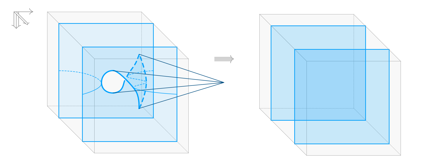
\[x_1^3 - x_2^2 x_1 + u_1 (x_2^2 + x_1^2) - u_2 x_2 - u_3 x_1.\]In [1] we describe a recipe for turning this unfolding into a tame tangle: namely, a tangle can be obtained from the hyper-surface $\tilde\Gamma_f$ of points $\{(u_3,u_2,u_1,f(x_1,x_2,u_1,u_2,u_3),x_2,x_1) \in \lR^6\}$, by appropriately restricting $\tilde\Gamma_f$ to a framed subcube $\II^6 \into \lR^6$ containing the origin. Note, the latter inclusion projects to a framed subcube $\II^3 \into \lR^3$: we visualize the situation (for a somewhat very “standard” looking inclusion) on the left in the Figure below.
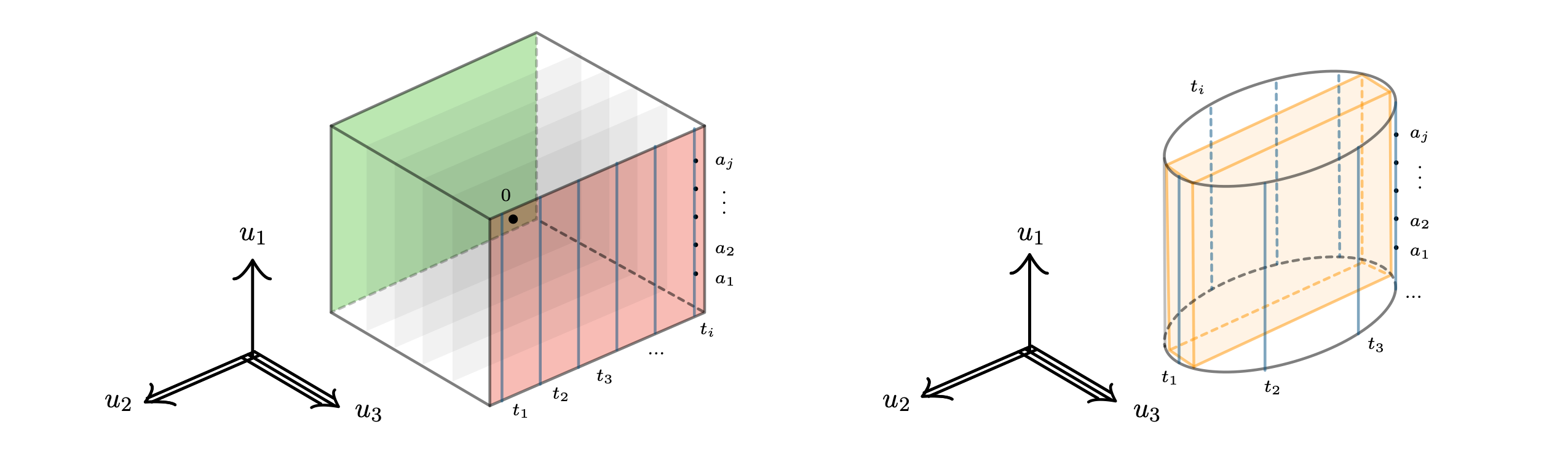
We’ll be interested in the link $L_f = \partial \II^3 \cap \tilde\Gamma_f$ of the singularity around the origin—as a tame tangle, this splits up into a source and target part: the face of the framed cube inclusion corresponding to source and target are highlighted in green resp. red in Fig. 1.
Note, each point in the source (resp. the target) face of the cube is described by a triple $\mathbf{u} = (u_1,u_2,u_3)$; fibered over each such point is the hyper-surface of $\tilde \Gamma_{f,\mathbf{u}}$ points $(f(x_1,x_2,u_1,u_2,u_3),x_2,x_1)$ in $\II^3$ which is a 2-tangle in the 3-cube. Varying the parameters $u_i$ evolves this 2-tangle making the source/target a 4-tangle in $\II^5$ (note the evolution is in two dimensions since $u_3$ is fixed for both source and target face: the categorical 4-direction evolution is the parameter $u_1$, and the 5-direction is the parameter $u_2$). To visualize these 4-tangles in $\II^5$ we can sample their $\II^4$ slices at different $u_2$-parameter “times” $t_1, …, t_i$, and at each such time, sample $\II^3$ slices of $\II^4$ slices at different $u_1$-parameter “times” $a_1, …, a_j$. This is schematically illustrated in the Fig. 1 (on the left) for the target.
It turns out we can further clarify the visualization of the $L_f$ if we change our plan slightly as follows: instead of sampling the source and target of a cube as shown above, we will sample our 4-tangle in $\II^5$ on the boundary a “cylinder” as shown on the right—technically, this cylinder is not the image of a framed embedding of a 3-cube $\II^3$; however, we could chose a thin framed-embedded cube (illustrated in orange) and this would lead us to a qualitatively similar visualization of $L_f$. Note that by sampling times $t_k$ “around the cylinder” we combine source and target 4-tangle into a single 4-tangle in $\II^5$, which we refer to as $L_f$. We are now ready to actually plot $L_f$.
The above plan to sample the hypersurfaces $\tilde \Gamma_{f,\mathbf{u}}$ at varying $\mathbf{u}$ is implemented by the following Mathematica code. Note, there are several choices of numerical values ($a$ times range between $[-1.5, +1.5]$, $t$ times between $[0, 2\pi]$, the cylinder radius is $1.5$, $x_i$ are plotted between $[-3,3]$, $f$ values between $[-40,40]$; note the monomial $x_1^3$ in $f$ is modified by a factor $\frac{1}{3}$; note also $i$ above becomes the variable slices4D below, and $j$ becomes slices3DPer4Dslice)—all of these choices are so that “the action becomes clearly visible”. The “action” can be seen in a movie below.
slices4D = 12;
slices3DPer4Dslice = 80;
movieFrame = 0;
While[
 movieFrame < slices4D*slices3DPer4Dslice,

 frameTuple = QuotientRemainder[movieFrame, slices3DPer4Dslice];
 t = frameTuple[[1]]*(2*Pi)/slices4D;
 a = -1.5 + frameTuple[[2]]*3/slices3DPer4Dslice;
 f[x_, y_] = (1/3)*x^3 - x*y^2 + a*(x^2 + y^2) -
   1.5*Cos[t]*y - 1.5*Sin[t]*x;
 criticalPoints = {x, y, f[x, y]} /.
   NSolve[{x^2 - y^2 + 2*a*x - 1.5*Sin[t] ==
      0, -2*x*y + 2*a*y - 1.5*Cos[t] == 0}, {x, y}, Reals];
 framePlot =
  Show[Plot3D[f[x, y], {x, -3, 3}, {y, -3, 3},
      PlotRange -> {-40, 40}, MeshFunctions -> {#3 &}, Mesh -> 100,
      BoxRatios -> {1, 1, 3},
      PlotStyle ->
       Directive[Yellow, Specularity[White, 20], Opacity[0.7]],
      ImageSize -> {1899, 1899}, ViewVector -> {80, -32, 560},
      ViewAngle -> -10, AxesLabel -> Thread@Text[{"x", "y", "f"}],
      PlotLabel ->
       Style[
        Framed[
         "time = " <>
          StringPadRight[ToString[NumberForm[N[t], 3]], 4, "0"] <>
          " height = " <>
          StringPadRight[ToString[NumberForm[N[a], 3]], 4, "0"]],
        16]],
     Graphics3D[{Red, PointSize[.005], Point[criticalPoints]}],
     Graphics3D[{Blue, PointSize[.005],
       Point[{#[[1]], #[[2]], 0} & /@ criticalPoints]}],
     Graphics3D[{Black, PointSize[.002],
       Point[{-3, -3, #[[3]]} & /@ criticalPoints]}]];
    Export["frame" <> StringPadLeft[ToString[movieFrame],
    4, "0"] <> ".jpg", framePlot];;

   movieFrame++]
The Mathematica code generates movie frames that can be assembled into a single movie watchable below—note that, really, it is a “movie of movies”: for each time $t_k$ there is a movie of hypersurfaces in $\II^3$ with a frame for each of the times $a_1, …, a_j$. For our later interpretation as a tangle, it is extremely helpful to also plot critical points (i.e. points $(x_1,x_2)$ where the $df = 0$): these are marked by red dots in the movie, while blue dots are the projection of red dots to the plane $\lR^2 \times 0 \subset \lR^3$ (this is helpful to “see” the value $f(x_1,x_2)$ at a critical point: its the distance between the red and the blue point).
In the paused video, you can navigate frames with “.” and “,” (press twice since the video has 12fps instead of the usual 24fps). Here’s a link to the original video file which should be yet better quality if you download it (~160MB).
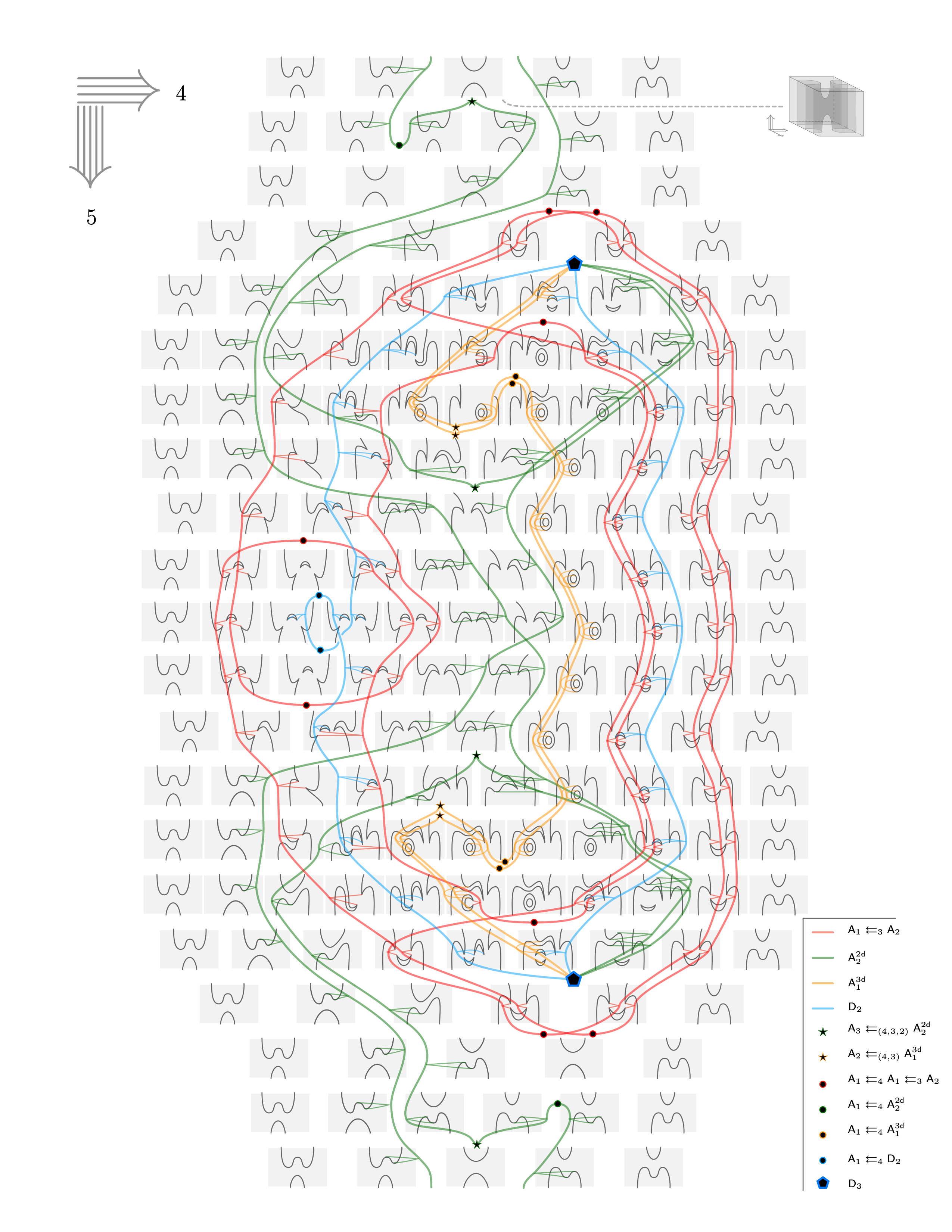
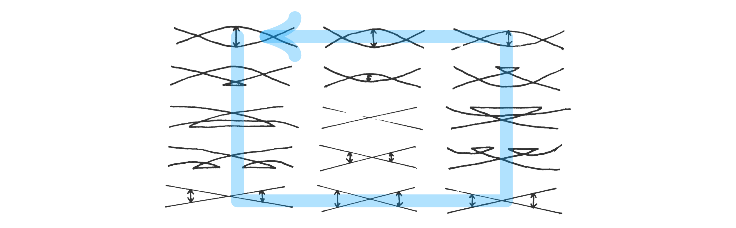
Note that these hypersurfaces in $\II^3$ aren’t actually 2-tangles yet: they do intersect the cube $[-3,3] \times [-3,3] \times [-40,40]$ badly on the boundary $\partial (3\II^2) \times [-40,40]$ (where $3\II^2 = [-3,3] \times [-3,3]$)—however, this is easily remedied by choosing a different framed cube (see Fig. 3.15 in [1] for how this is done in the case of the saddle 2-tangle), and we are allowed to vary this cube frame-by-frame (by definition of framed maps). Doing so leads to a movie of movies of 2-tangles, and this is illustrated in the next Figure—in order to be able to read this Figure not the following.
- Rows are evolution in categorical 4-direction (i.e. increasing time $a$)
- Columns evolve rows in categorical 3-direction (i.e. increasing time $t$)
- To depict individual 2-tangles in $\II^3$ we use shorthand notation by projecting to critical 2-tangles to $\II^2$, see Section 3.4 in [1]. This requires an “initial condition” which is given in the lower left of the Figure.
- All 2-tangle data is given in shades of grey.
- Thin colored lines indicate evolution in 4-direction.
- Thick colored lines indicate evolution in 5-direction—in fact, thick colored lines are line strata in the manifold diagram corresponding to the 4-tangle (see Section 3.1 in [1])).
- Colored dots are point strata in the manifold diagram corresponding to the 4-tangle.
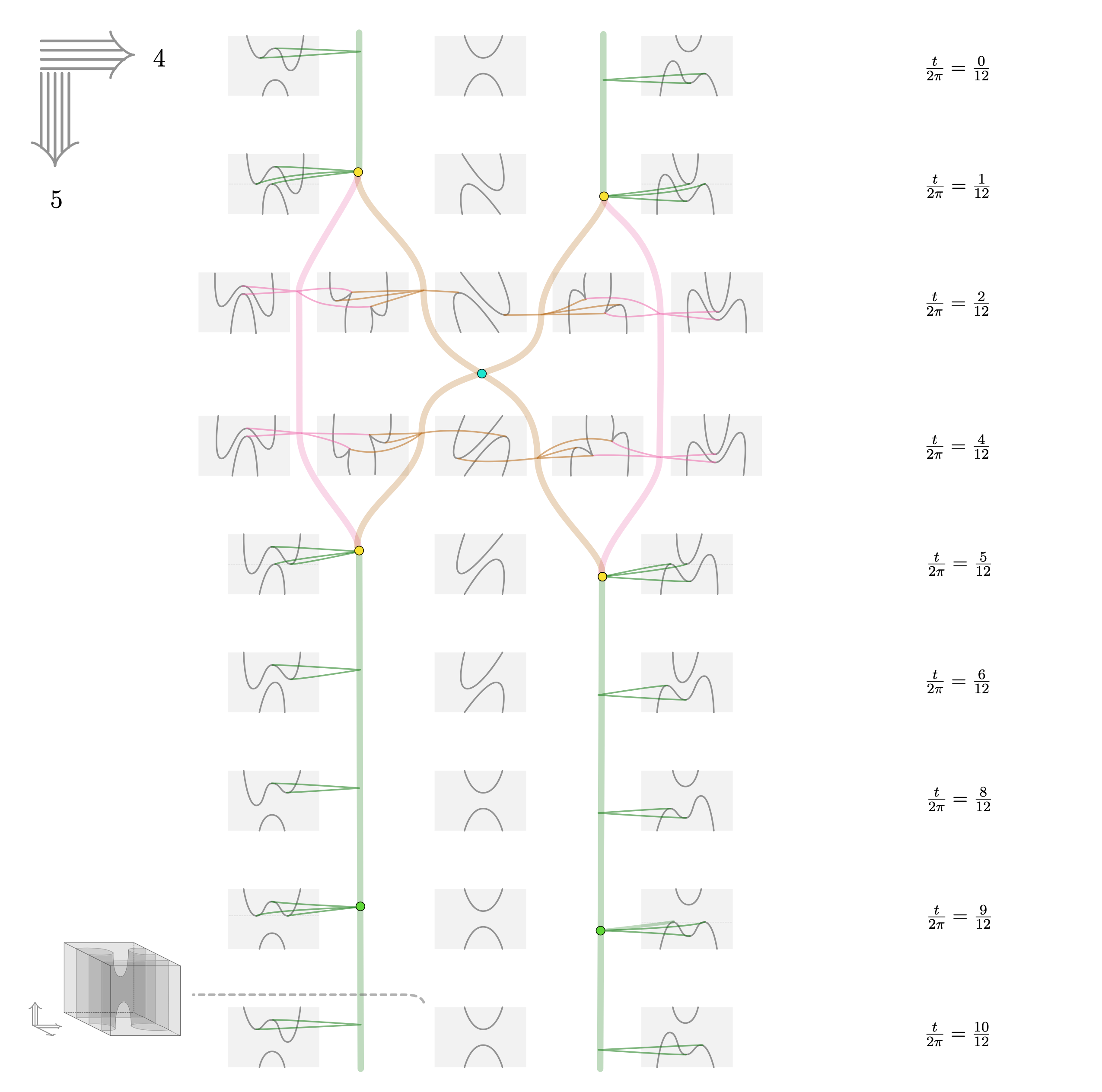
Before heading to the next section, we pat ourselves on the shoulder for having chosen slices4D = 12: indeed, from the above we see that interesting deformations happen for times $\frac{t}{2\pi}$ being $\frac{1}{12}$, $\frac{3}{12}$, $\frac{5}{12}$, and $\frac{9}{12}$ (Note 1: for $\frac{7}{12}$ and $\frac{11}{12}$ stuff happens too as “things move past each other”, but this is somewhat less interesting) (Note 2: the event at $\frac{3}{12}$ is similarly invisible from just looking at critical points in the movie, but only appears when working with framed space). Compare this to the classical “3-fold” symmetry in the parameter space of the $D^-_4$ singularity which can be seen e.g. here.
Perturbing the link to generic form
Taking the cone of the 4-tangle $L_f$ in Fig. 2 defines a 5-tangle singularity which in [1] we denoted by $\iD_4$. As discussed there, the singularity appears to be stable—but it is not inductively stable: that is, the link $L_f$ uses tangle singularities that can be perturbed into simpler tangle singularities. We now outline how such a perturbation can be achieved.
As a first step, recall [1] classes of stable 3-tangle singualarities that can be constructed as “binary algebraic relators” of lower-dimensional singularities: we reillustrate these classes in Fig. 3 below. It will turn out that 3-tangle singularities of these “binary” types (and analogous “binary” 4-tangle singularities) suffice to write down a perturbation of $L_f$.
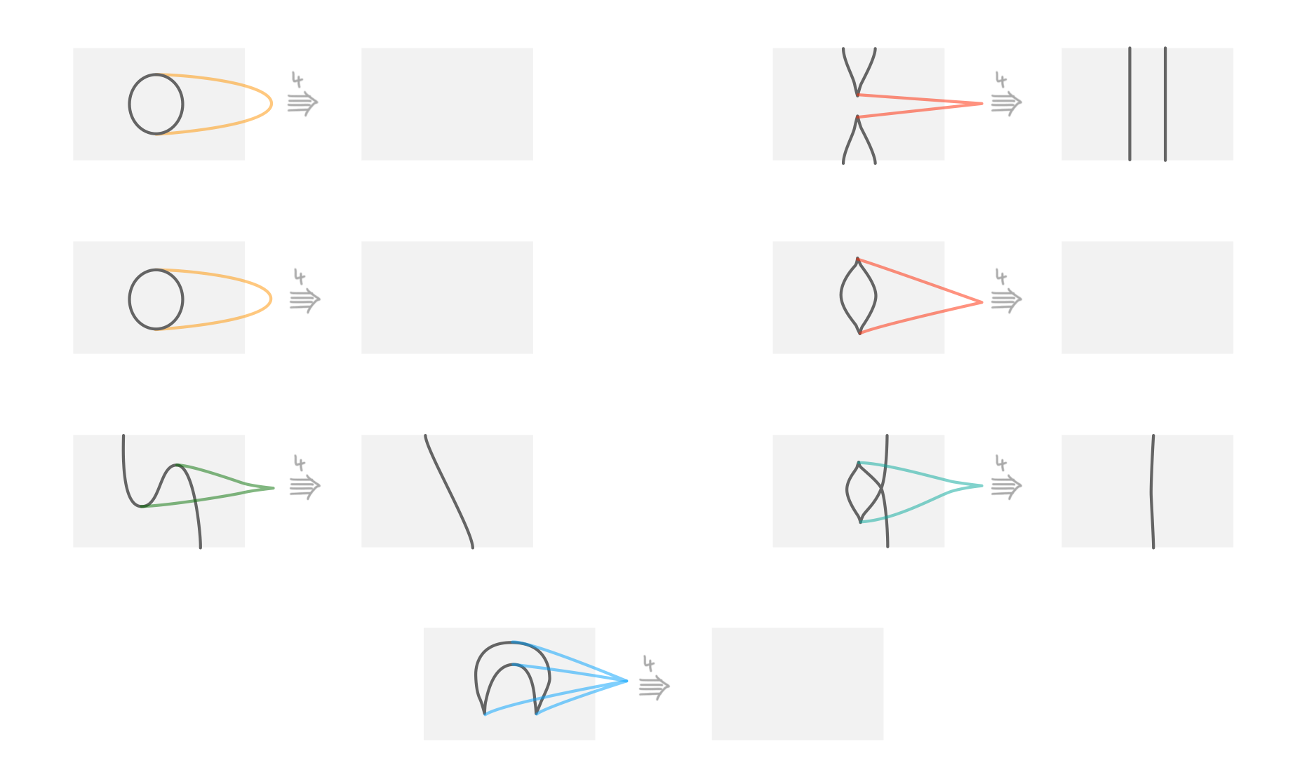
Take note of the colors chosen for these singularities: we will use them consistently in the following, for indicating singularities from classes represented by those in Fig. 3.
As a first step in perturbing $L_f$ consider the (thick) pink and brown line strata in Fig. 2: let us call the pink singularity the “morse-split” and the brown singularity the “cusp-kiss”. Neither of these singularities are stable—the fact that they can be perturbed into simpler singularities is illustrated in Fig. 4 below.
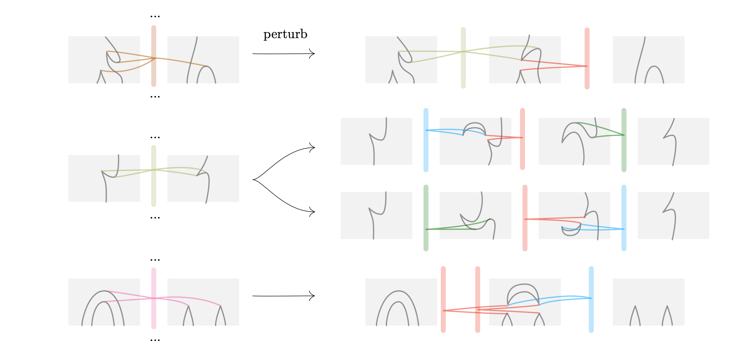
In the first line, we perturb the cusp-kiss into two separate lines: the “cusp-flip” (the term frequently occurs in work on diagrammatic algebra) and the red singularity from Fig. 3. In the next line, we record two reasonable perturbations of the of the cusp-flip: one ends in the color sequence blue-red-green and the other in the (reverse sequence) green-red-blue. The fact that there are two such perturbations, will be important in a moment. In the last line, we perturb the morse-split into three singularities (yielding a red-red-blue sequence).
Our approach to perturbing $L_f$ will first perturb line strata, splitting them up into multiple line strata as shown in Fig. 4. In fact, this will also naturally lead to splittings of point strata as we will see. However, The “figure 8” in $L_f$ around the time $\frac t {2\pi} = \frac 3 12$ leads to a complication that will require as to reverse the color-sequence blue-red-green into the sequence green-red-blue. This reversal requires additional singularities (which turn out to be crucial!) as illustrated by a “zoomed-in part” in the next figure: this figure depicts a first perturbation of the link $L_f$. Note that our depiction is schematic: except for the zoomed in part, it only depicts global 4-5-structures, leaving the full 1-2-3-4-5-structure to be filled in by the reader (of course we claim there is just one correct way of doing it).
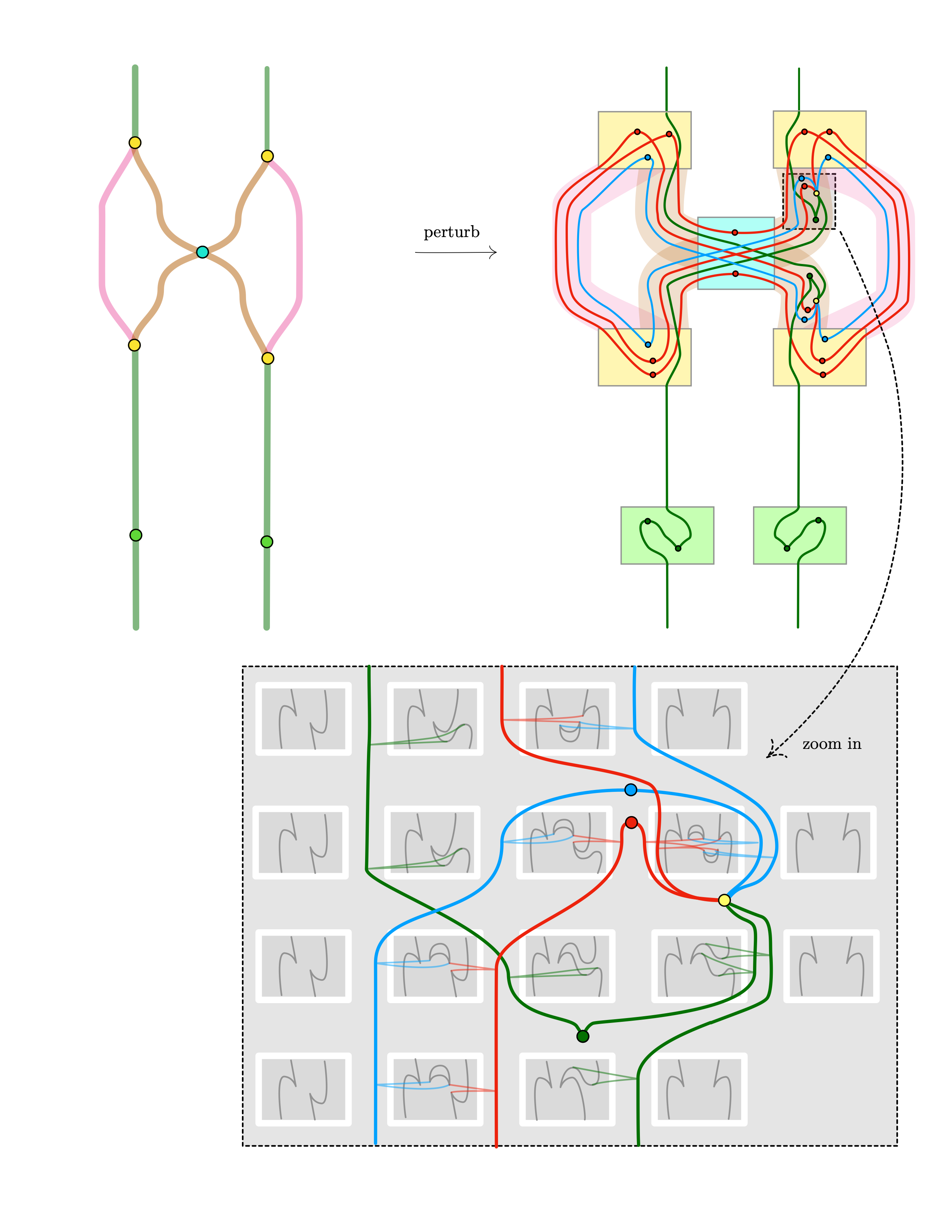
Fig. 5 shows a 4-tangle $L^\prime_f$ that perturbs our earlier tangle $L_f$. $L^\prime_f$ is almost stable: namely, it is perturbation stable except for the box in the color-sequence reversal—the yellow point stratum (yellow dot) is a tangle singularity that is in fact not yet stable. Thus in the next step is to perturb the yellow point stratum. We forego producing another image for this perturbation: the perturbation will precisely contain an $\iD_3$ that also appears in the next figure (and the remaining details are once more left to the reader). Instead, let us fast forward: perturbing the yellow singularity leads to another perturbation $L^\prime_f \rightharpoonup L^{\prime\prime}_f$. Now, $L^{\prime\prime}_f$ can be further simplified by an isotopy path $L^{\prime\prime}_f \to \tilde L_f$, which allows to remove some point and line and strata from the above (note that we don’t claim that our choice of perturbation or subsequent isotopy is unique). The resulting tangle $\tilde L_f$ is thus $\mathscr{F}$-equivalent to the link $L_f$ we started with, and thus the cone $\tilde\iD_4$ of $\tilde L_f$ is $\mathscr{F}$-equivalent to $\iD_4$ (making $\tilde\iD_4$ and $\iD_4$ appropriately equivalent as tangle singularities). The link $\tilde L_f$ is shown in the next and final figure (Note: for added symmetry, one of the two bottom green boxes in $L^\prime_f$ in Fig. 4 was moved to the top of $\tilde L_f$ in Fig. 5).
The final product
Let us cast the $D_4$ link into even nicer form by “taking the trace”. For this we bend the two green lines in Figure 5 around from the target into the source: after minor further simplification, the result is shown in Figure 6 below (again, this only depict the 4-5 structure with the same orientation as before; note also that thicker lines are meant to abbreviate double lines of the same color from the previous figure).
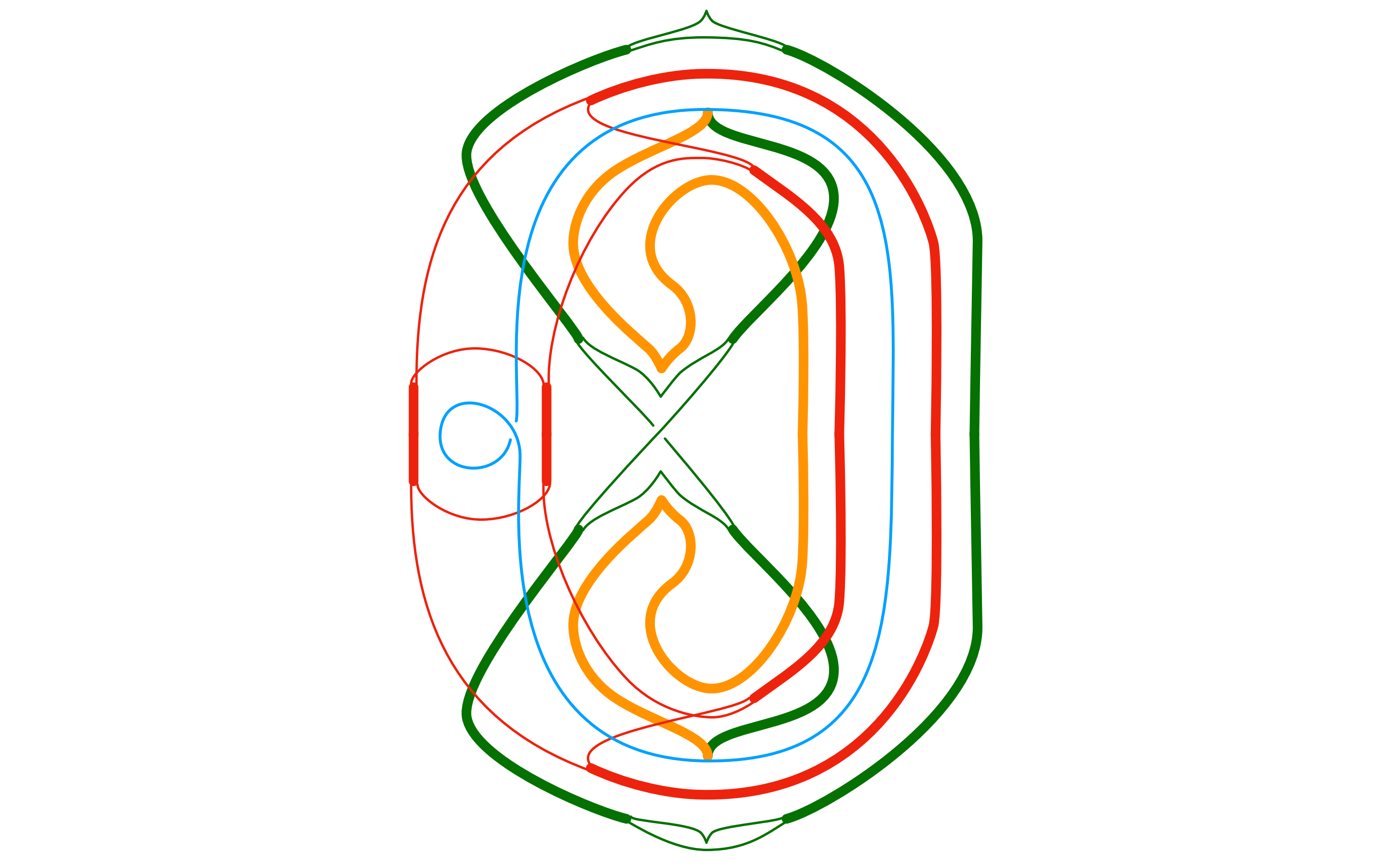
Ignoring all but the green and blue lines (and switching the outer green two cups and two cusps respectively into a parallel position), we may take the cone of this picture to arrive at Figure 6b below.
(As an aside: for a loose point of comparison, consider the $A_3$-like 4-singularity in Figure 6c, which indicates (albeit in a different topological setting) how we may think of the blue lines in the 6-singularity of Figure 6b.)
The core observation made in [1] is the following: the above shows that $\tilde\iD_4$ can be perturbed to an algebraic binary relator of $\iD_3$ singularities. This expresses a binary law of $\iD_3$ singularities, just as a the simple $A_2$ singularity corresponds to the usual law for units and counits (i.e. $\iA_1 = \iM_1$ singularities) in adjoints. This gives a first idea of a much larger interaction of coherent dualizability laws and classical singularities (respective their combinatorial re-casting in terms of tame tangle singularities as developed in ).
Further notes
Hatcher-Wagoner $D_4$ in Cerf graphics
I recently found another depiction of the $D_4$ singularity in work of Hatcher and Wagoner in terms of Cerf graphics: namely, Figure (6) on page 202 of [5]. The picture nicely shows six swallowtail-type singularities in the link of the $D_4$ singularity. These six points correspond to the two green and four yellow points in Fig. 2. We now explain this in detail.
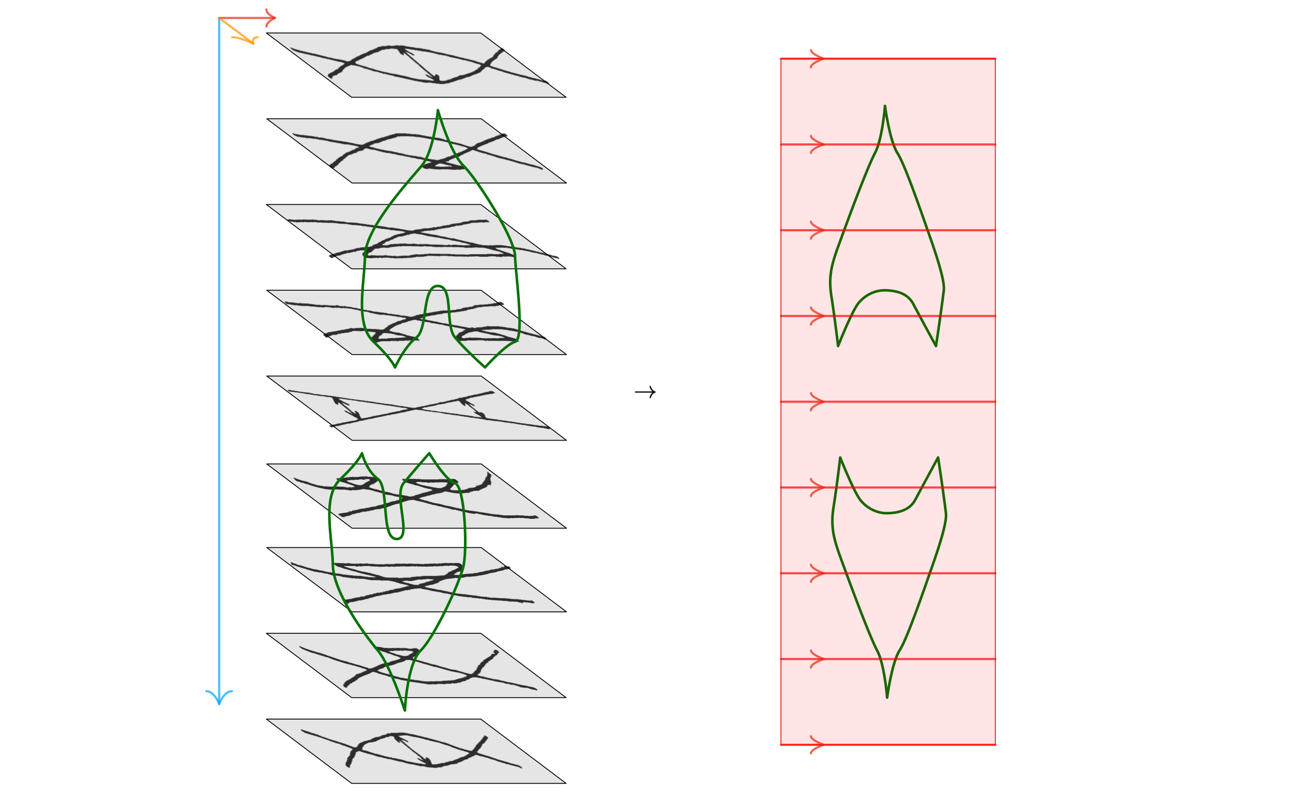
Let us first extend Hatcher and Wagoner’s graphic a little bit. In Figure 7 below, we copied Figure (6) on page 202 from [5], which depicts the $D_4$ singularity as a series of Cerf graphics. We are interested in the link of the $D_4$ singularity, so let us walk around the outer Cerf graphics as indicated by the thick blue arrow.
This yields a “movie of Cerf grapics” as shown on the left in Figure 8 below. Let us now frame this movie: the direction of the movie (blue arrow) will be our 5th categorical direction, the path-direction of individual Cerf graphics (red arrow) will be our 4th categorical dimension, and the Morse-direction of individual Cerf graphics (orange arrow) will be our 3rd categorical direction. We now overlay the movie with the loci of cusps by green lines. Note these lines themselves have cuspidal points, and these points represent swallowtail-type singularities. Now let’s project these loci to the categorical 4-5 plane: this yields the picture shown on the right.
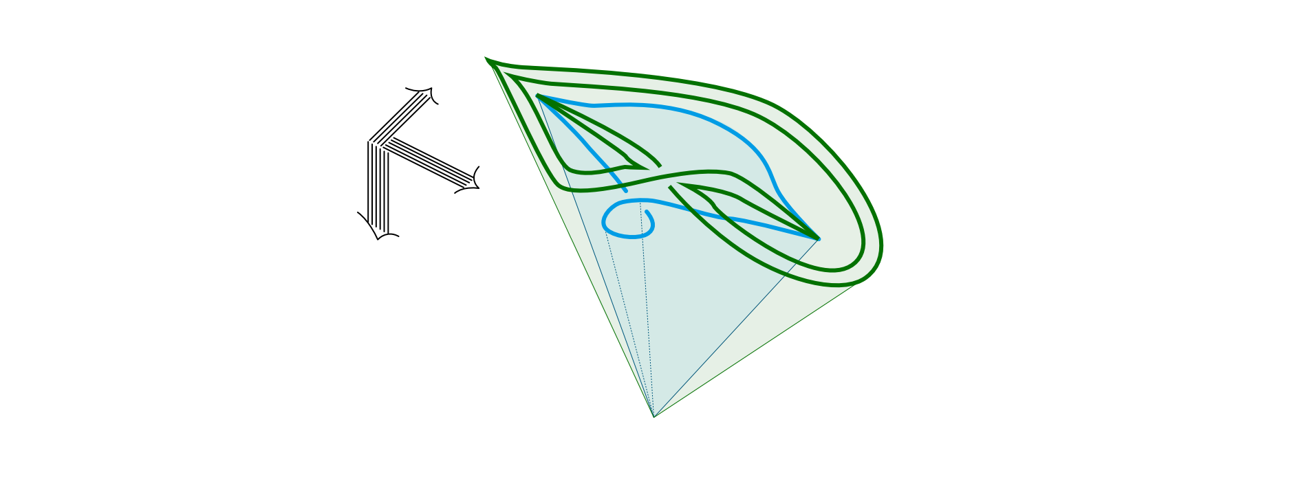
The resulting projected picture in Figure 8 can now be thought about (and compared to our pictures) as follows. Consider a link sphere around the $D_4$ singularity; in the 3-dimensional parameter space, this is a 2-sphere. The sphere may be framed (or foliated) in several ways, two of which are shown in Figure 9 below. (Framings are indicated by both red and blue arrows, whereas the green stratification shows the singular loci of the $D_4$ singularity projected to its parameter space — this reproduces the usual picture drawn for the $D_4$ singularity.) Flattening the intersection of the singular loci of $D_4$ with the framed sphere produces two different pictures shown on the right: the first recovers Hatcher and Wagoner’s picture in Figure 8, and the second recovers our Figure 2, after only remembering the cusp loci, i.e. the green and pink lines (the pink line is a sort of “sideways” cusp; the difference to the “normal” cusp, represented by the green line, only arises in the higher parameter setting of tame tangles).
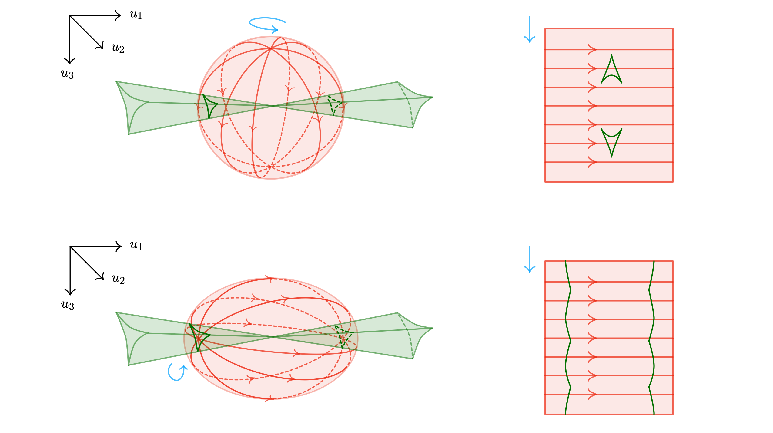
This comparison makes it clear that the six swallowtail-type singularities of Figure 8, reappear in our earlier Fig. 2 as the six singularities given by the two green and four yellow points.
Moreover, the two pictures are related by a deformation of the sphere framing (a pretty simply one; just rotate the sphere). Categorically, this deformation alters the source and target of the $D_4$ singularity by bending wires from one into the other (fully analogous to how we obtained Figure 6 from Figure 5 earlier). The two choices of framing in the parameter space link are therefore equivalent (i.e. categorically equivalent, up to using the various singularities required for the bending). The reason we prefer our framing over Hatcher and Wagoner’s choice is that it better aligns with the symmetry of the $D_4$ singularity, and makes the representation of “higher parameter behaviour” (e.g. the brown lines in Figure 2) simpler.
Fiber bundle perturbations
Technically, [1] introduces two notions of perturbations: stratified perturbations (which are stratified bundles, and may change the local topology of tangles), and fiber bundles perturbations (which do not change the local (and thus global) topology of tangle fibers). All perturbations in this note are of the latter type. In fact, whenever one works in codimension-1, it is natural to work with fiber-bundle perturbations, while in higher codimension “unstable” differences between the two notions arise (see Rmk. 3.3.8 in [1]).
References
[1] “Manifold diagrams and tame tangles”, Dorn + Douglas
[2] Local normal forms of functions, V Arnold
[3] Notes on the classification of singularities, CTC Wall
[4] Singularities of mappings, D Mond + JJ Nuno-Ballesteros
[5] Pseudo-isotopies of compact manifolds, Hatcher + Wagoner