Mazur manifold as tangle diagram

<! --- LETTERS ---> $$ \newcommand{\lR}{\mathbb{R}} $$ $$ \newcommand{\lZ}{\mathbb{Z}} $$ $$ \newcommand{\lN}{\mathbb{N}} $$ $$ \newcommand{\lI}{\mathbb{I}} $$ $$ \newcommand{\II}{\mathbb{I}} $$ $$ \newcommand{\bI}{\mathbf{I}} $$ $$ \newcommand{\bC}{\mathbf{C}} $$ $$ \newcommand{\bD}{\mathbf{D}} $$ $$ \newcommand{\bE}{\mathbf{E}} $$ $$ \newcommand{\bF}{\mathbf{F}} $$ $$ \newcommand{\iI}{\mathsf{I}} $$ $$ \newcommand{\iA}{\mathsf{A}} $$ $$ \newcommand{\iB}{\mathsf{B}} $$ $$ \newcommand{\iC}{\mathsf{C}} $$ $$ \newcommand{\iD}{\mathsf{D}} $$ $$ \newcommand{\iE}{\mathsf{E}} $$ $$ \newcommand{\iF}{\mathsf{F}} $$ $$ \newcommand{\iM}{\mathsf{M}} $$ <! --- SYMBOLS ---> $$ \newcommand{\eps}{\epsilon} $$ $$ \newcommand{\SetCat}{\mathrm{Set}} $$ $$ \newcommand{\Bool}{\mathrm{Bool}} $$ $$ \newcommand{\Pos}{\mathrm{Pos}} $$ $$ \newcommand{\lbl}{\mathsf{lbl}} $$ $$ \newcommand{\subdiv}{\mathsf{sd}} $$ $$ \newcommand{\Hom}{\mathrm{Hom}} $$ $$ \newcommand{\Fun}{\mathrm{Fun}} $$ $$ \newcommand{\Psh}{\mathrm{PSh}} $$ <! --- OPERATORS ---> $$ \newcommand{\dim}{\mathrm{dim}} $$ $$ \newcommand{\id}{\mathrm{id}} $$ $$ \newcommand{\src}{\partial^-} $$ $$ \newcommand{\tgt}{\partial^+} $$ $$ \newcommand{\und}[1]{\underline{#1}} $$ $$ \newcommand{\abs}[1]{\left|{#1}\right|} $$ $$ \newcommand{\op}{^{\mathrm{op}}} $$ $$ \newcommand{\inv}{^{-1}} $$ <! --- CATEGORIES, FUNCTORS AND CONSTRUCTIONS ---> $$ \newcommand{\ttr}[1]{\mathfrak{T}^{#1}} $$ $$ \newcommand{\lttr}[2]{\mathfrak{T}^{#1}{(#2)}} $$ $$ \newcommand{\truss}[1]{\mathsf{T}\!\mathsf{rs}_{#1}} $$ $$ \newcommand{\sctruss}[1]{\bar{\mathsf{T}}\!\mathsf{rs}_{#1}} $$ $$ \newcommand{\rotruss}[1]{\mathring{\mathsf{T}}\!\mathsf{rs}_{#1}} $$ $$\newcommand{\trussbun}[1]{\mathsf{TrsBun}_{#1}} $$ $$ \newcommand{\trusslbl}[1]{\mathsf{Lbl}\mathsf{T}\!\mathsf{rs}_{#1}} $$ $$ \newcommand{\blcat}[1]{\mathsf{B}\mathsf{lk}_{#1}} $$ $$ \newcommand{\blset}[1]{\mathsf{Blk}\mathsf{Set}_{#1}} $$ $$ \newcommand{\fcl}[2]{\chi^{#1}_{#2}} $$ $$ \newcommand{\Entr}{\mathsf{Entr}} $$ $$ \newcommand{\Exit}{\mathsf{Exit}} $$ <! --- ARROWS AND RELATIONS ---> $$ \newcommand{\fleq}{\preceq} $$ $$ \newcommand{\fles}{\prec} $$ $$ \newcommand{\xto}[1]{\xrightarrow{#1}} $$ $$ \newcommand{\xot}[1]{\xleftarrow{#1}} $$ $$ \newcommand{\ot}{\leftarrow} $$ $$ \newcommand{\toot}{\leftrightarrow} $$ $$ \newcommand{\imp}{\Rightarrow} $$ $$ \newcommand{\iff}{\Leftrightarrow} $$ $$ \newcommand{\iso}{\cong} $$ $$ \newcommand{\into}{\hookrightarrow} $$ $$ \newcommand{\proto}{\longrightarrow\mkern{-2.8ex}{\raisebox{.3ex}{$\tiny\vert$}}\mkern{2.5ex}} $$ <! --- DIAGRAM ARROWS ---> <! ---... should replace \rlap by \mathrlap, see KaTeX doc ---> $$ \newcommand{\ra}[1]{\xrightarrow{\ \ #1\ \ }\phantom{}\kern-1.5ex} $$ $$ \newcommand{\la}[1]{\xleftarrow{\ \ #1\ \ }\phantom{}\kern-1.5ex} $$ $$ \newcommand{\da}[1]{\downarrow\raisebox{.5ex}{\rlap{$\scriptstyle#1$}}} $$ $$ \newcommand{\dra}[1]{\raisebox{.2ex}{\llap{$\scriptstyle#1$}}\kern-.5ex\searrow}} $$ $$ \newcommand{\dla}[1]{\swarrow\kern-1ex\raisebox{.2ex}{\rlap{$\scriptstyle#1$}}} $$ $$ \newcommand{\ua}[1]{\uparrow\raisebox{.2ex}{\rlap{$\scriptstyle#1$}}} $$ $$ \newcommand{\ura}[1]{\raisebox{.2ex}{\llap{$\scriptstyle#1$}\kern-.5ex\nearrow}} $$ $$ \newcommand{\ula}[1]{\nwarrow\kern-1ex\raisebox{.2ex}{\rlap{$\scriptstyle#1$}}} $$

Abstract. Mazur manifolds are intimately related to homology spheres, and are part of the puzzling world of 4-manifolds. Here we construct the simplest example of a Mazur manifold as a tangle diagram.

Introduction

The world of 4-manifolds can be quite puzzling. A part of this puzzle is the story of homology 3-spheres, and the question which 4-manifolds bound such homology spheres. For instance, every homology $n$-sphere, $n \geq 4$, smoothly bounds a contractible smooth compact manifold: a higher Mazur manifold. Moreover, the double of such Mazur manifolds is the $S^{n+1}$ sphere, and this means, after removing a point of $S^{n+1}$, that all such homology $n$-spheres smoothly embed in $\lR^{n+1}$ bounding a Mazur manifold (this may also be interpreted as part of a ‘Homology Schoenflies Theorem’). For $n = 3$, there is a different story. The ‘standard’ Poincare homology sphere (i.e. the Brieskorn sphere $\Sigma(2,3,5)$) does not bound a Mazur manifold, and it does not smoothly embed in $\lR^{4}$. However, a wild topological embedding into $\lR^4$ exists. This follows from Freedman’s result that all homology 3-spheres bound a contractible topological fake 4-ball, see (2.3 in [2]). (The result is crucial for the classification of topological 4-manifolds, and, e.g., for the construction of the $E_8$ manifold, see (2.4 in [2])).

The world of manifold and tangle diagrams is tame. In particular, there is no chance that the wild embedding $\Sigma(2,3,5) \into \lR^4$ can be made into a tangle diagram. However, there are smooth Mazur 4-manifolds, and these do bound homology 3-spheres. One homology 3-sphere that bounds a Mazur manifold in this way is $\Sigma(2,5,7)$. In this post we will describe a tangle diagram for the embedding $\Sigma(2,5,7) \into \lR^4$.

The tame tangle

Recall, 4-diagrams are often depicted as movies of 3-diagrams. In particular, this will apply to our 3-tangle 4-diagram. We will use stable singularities (or singularities closely related to stable ones) in our representation of the diagrams. A discussion of stability can be found in [1] and in this note on the $D_4$ singularity. With this in mind a depiction of the tangle 4-diagram $\Sigma(2,5,7) \into \lR^4$ is given in Figure 1 below: note the figure is a single movie, i.e. sequence of framed, but the sequence is broken up into multiple lines… read left-to-right, and top-to-bottom.

Figure 1: a tangle diagram for the embedding \(\Sigma(2,5,7) \into \lR^4\).

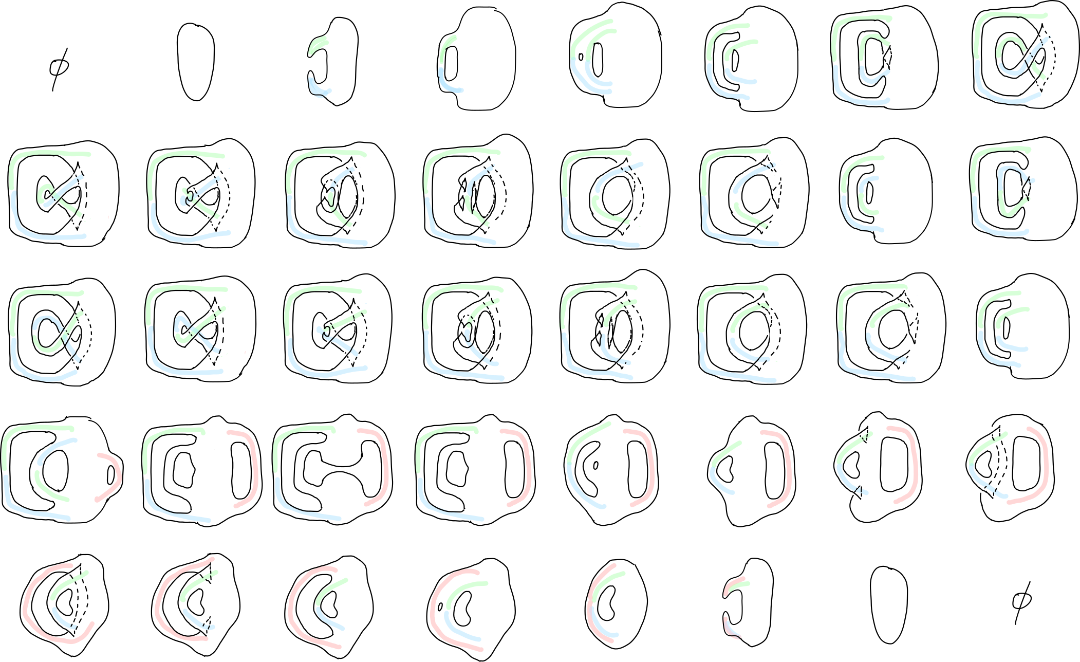
Colors in the picture may be ignored for now, even though they’ll be used later: they indicate handle attachments corresponding to the usual pictures drawn for Kirby diagrams (see Figure 4 for a Kirby diagram with colors that match those above).

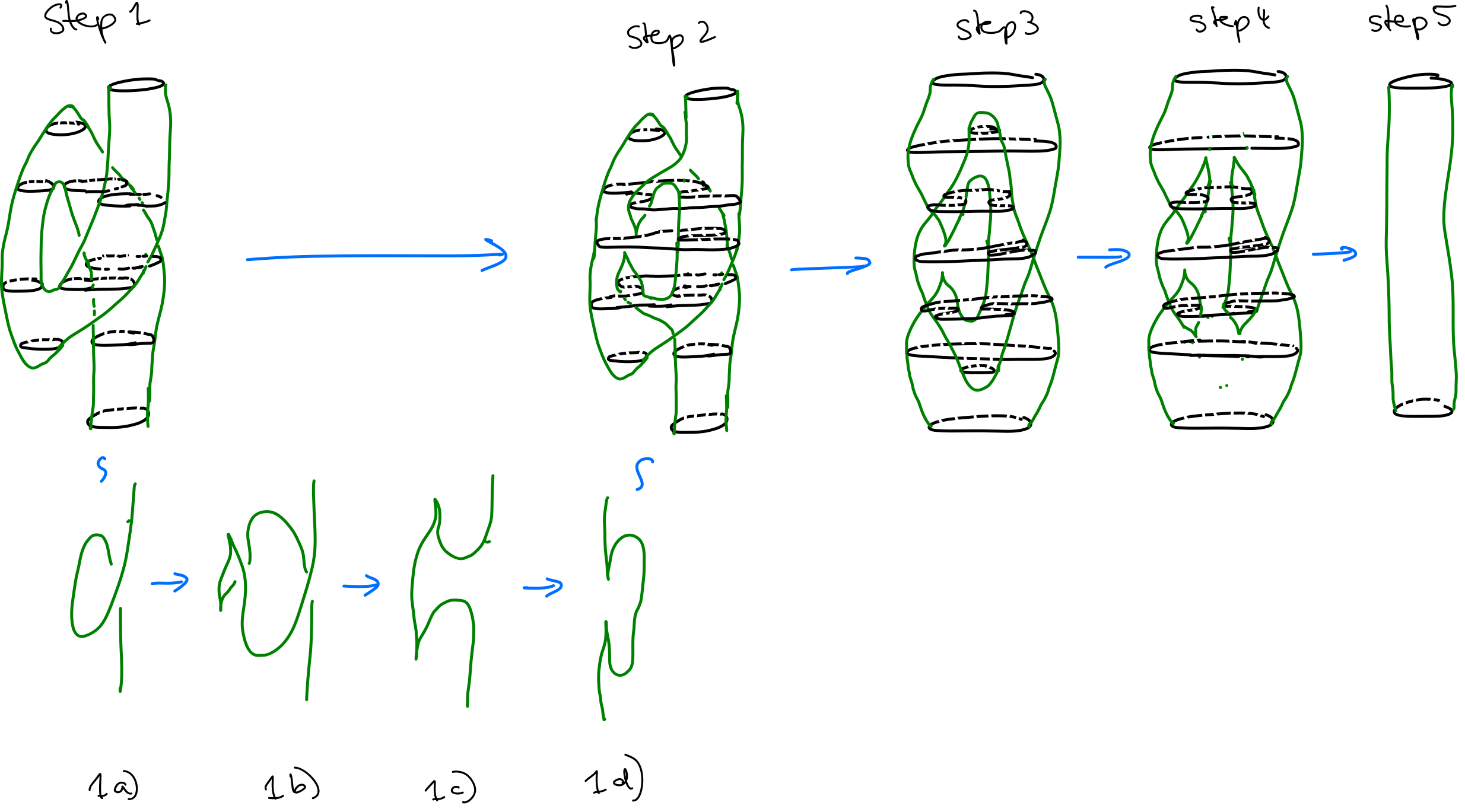
One crucial part of the movie in Figure 1 is the ‘double rotation’ of the inner green-blue tube. In Figure 2 below we illustrate in more detail how such a rotation looks like.

Figure 2: how to resolve a Serre tube to the identity.

The (1,2)-structure

The movie in Figure 1 is nice, but long. In Figure 3 we put the entire movie into a single picture, which could be thought of as its Morse-Cerf graphic—or its ‘(1,2)-Morse graphic’. Importantly, similar to traditional Cerf graphics, the image only records loci of Morse singularities in a 1-parameter family of Morse functions. That is, is does not ‘see’ higher singularities (such as the cusps in the movie frames in the movie of Figure 1). In two places of Figure 3, we ‘zoom in’ and illustrate how the full tangle structure in $\lR^4$ interplays with this 2-dimensional representation.

Figure 3: the \((1,2)\)-Morse structure of the homology 3-sphere embedding.

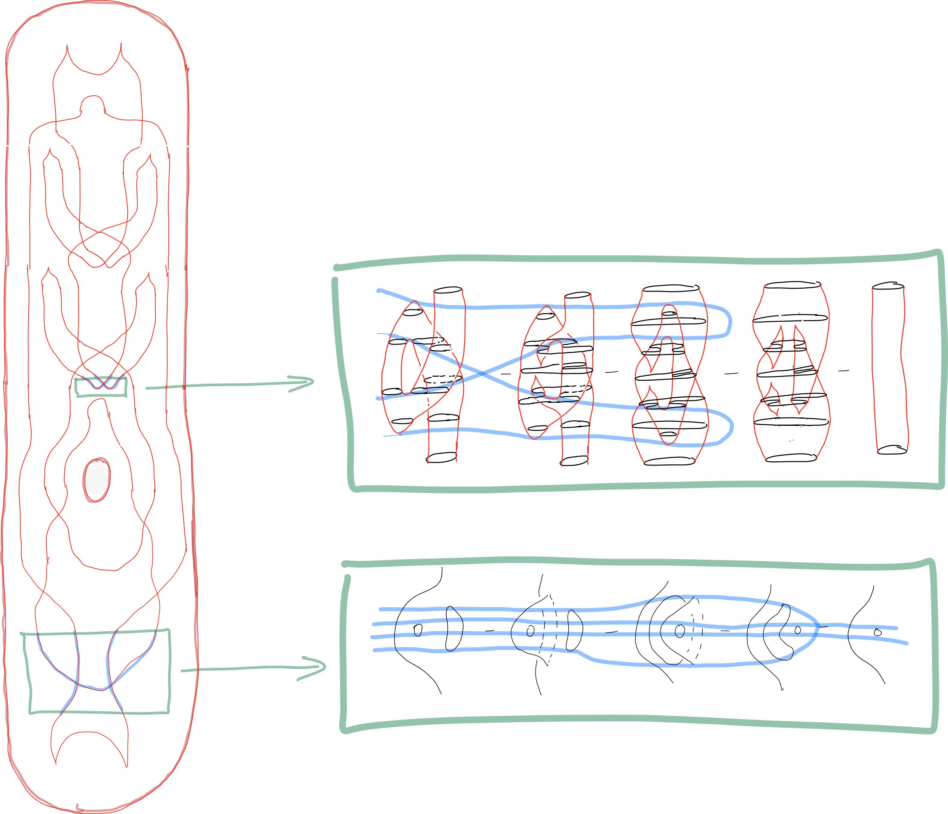
It may be worth noting that the second ‘zoom area’ in Figure 3 plays an important role. ‘Pulling one handle over another’ in this way is related to a family of higher singularities, which, in the heuristic notation of [1] would be denoted by $\mathsf{A} _ 3 \leftleftarrows_{(4,3,1)} \mathsf{A} _ 1 ^\mathrm{2d}$.

Comparison to Kirby Diagram

Let us compare the Morse-Cerf structure of our Mazur tangle to the Kirby diagram which is usually used to represent this manifold. This comparison is made in Figure 4 below.

Figure 4: the 2-Morse structure of \(W\) and the corresponding Kirby diagram.

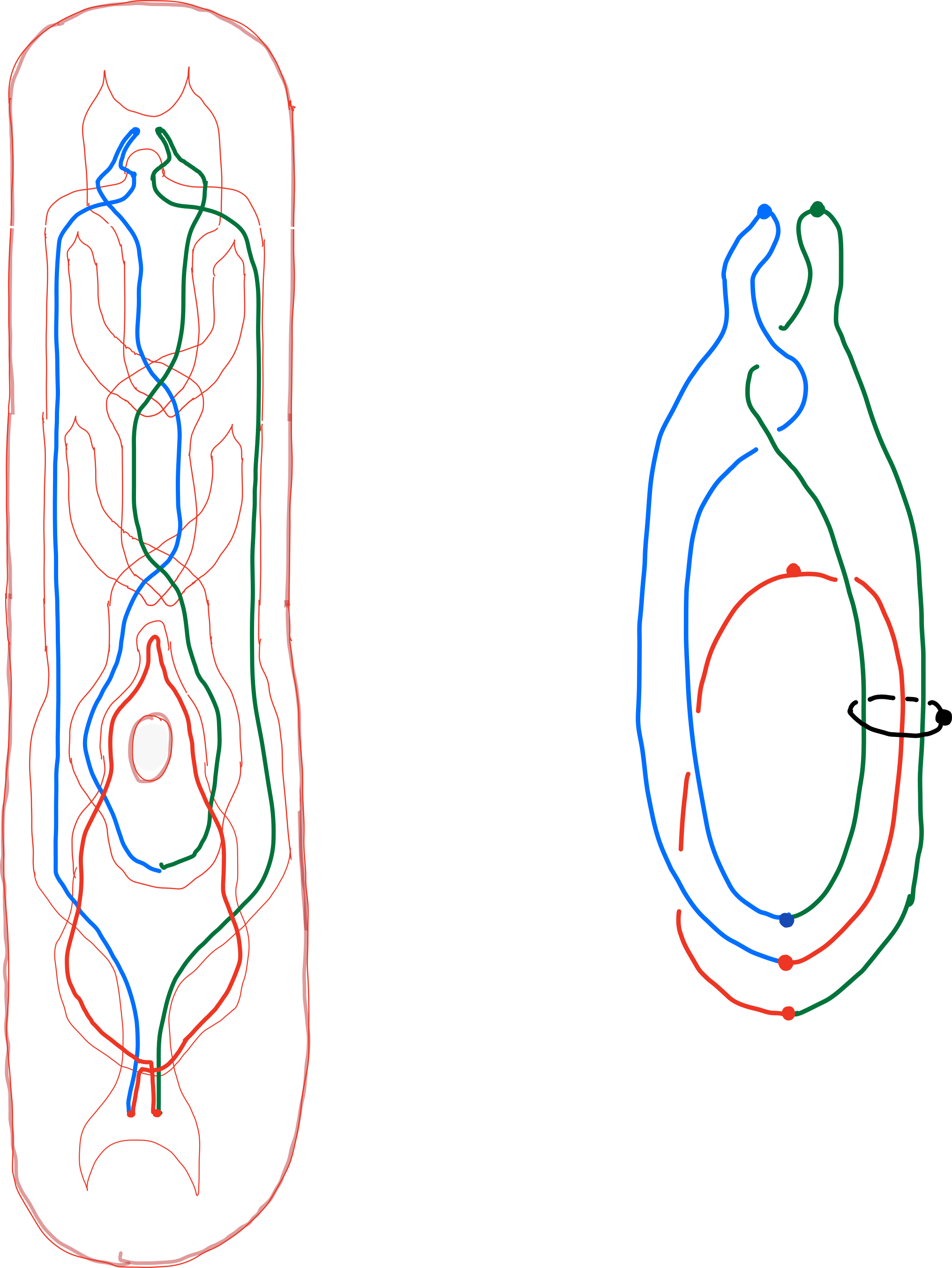
You can ignore colors (and colored dots) in order to read the Kirby diagram on its own—these have only been added for comparison with the 2-Morse picture on the left. The 2-Morse picture is augmented with colored lines mirroring those of the Kirby diagrams … the role of these lines is to indicate the ‘attachment’ points of handles (see Figure 1 for a color-coded depiction of those handles).

But why?

The codimension-1 case is special (see also the story of invertible morphisms). For instance, PL and smooth structures coincide in this case (up to choosing compatible normal framings). Moreover, in dimension $\neq 4$, homeomorphism and diffeomorphism also interplay better: all smooth topologically standard spheres are in particular smoothly standard spheres. In other words, the following statement holds in all dimensions but (potentially) $4$.

Smooth Poincare conjecture in codimension 1. A smooth homotopy $n$-sphere $W \into \lR^{n+1}$, $n \neq 4$, is diffeomorphic to the standard $n$-sphere.

The remaining case, $n = 4$, is a big open problem (note, for $n = 4$ the codimension-1 is equivalent to the general case, as explained e.g. in work by Colding-Minicozzi). If you solve it, you will likely win a Fields Medal. Until now, 1- and 2-Morse theoretic approaches seem to not have gotten us very far in really understanding what’s going on with smooth homotopy $4$-spheres. Stable tangle diagrams can be thought of as $n$-Morse decompositions of their tangle manifolds, and this provides us with a (higher-)algebraic description of the geometry at issue. In codimension 1, the perturbation-stable singularities of such tangles seem tractable, and closely related to differential ADE singularities. Eventually, understanding these singularities and their algebra (thus generalizing ‘handle cancellations’ to higher parameter dimensions), might help resolve the missing $n = 4$ case above. The singularity $\mathsf{A} _ 3 \leftleftarrows_{(4,3,1)} \mathsf{A} _ 1 ^\mathrm{2d}$ mentioned earlier is part of this story (and so is, one dimension up, the $D_4$ singularity).

Looking at the case $n = 3$ is instructive since a lot of new behaviour appears in this dimension. In particular, the above representation of a homology 3-sphere yields the question how it may be distinguished from the standard 3-spheres based on its higher Morse data (of course, the data may be represented 3-dimensionally in a Kirby diagram which provides one answer, but that answer doesn’t easily generalize to higher dimensions!). It is interesting to remove the ‘double tube rotation’ from our tangle—the result is indeed $S^3$ as can be shown by a sequence of ‘higher handle cancellations’!

References

[1] “Manifold diagrams and tame tangles”, Dorn + Douglas

[2] The wild world of 4-manifolds, Scorpan