The class of computadic cells

<! --- LETTERS ---> $$ \newcommand{\lR}{\mathbb{R}} $$ $$ \newcommand{\lZ}{\mathbb{Z}} $$ $$ \newcommand{\lN}{\mathbb{N}} $$ $$ \newcommand{\lI}{\mathbb{I}} $$ $$ \newcommand{\II}{\mathbb{I}} $$ $$ \newcommand{\bI}{\mathbf{I}} $$ $$ \newcommand{\bC}{\mathbf{C}} $$ $$ \newcommand{\bD}{\mathbf{D}} $$ $$ \newcommand{\bE}{\mathbf{E}} $$ $$ \newcommand{\bF}{\mathbf{F}} $$ $$ \newcommand{\iI}{\mathsf{I}} $$ $$ \newcommand{\iA}{\mathsf{A}} $$ $$ \newcommand{\iB}{\mathsf{B}} $$ $$ \newcommand{\iC}{\mathsf{C}} $$ $$ \newcommand{\iD}{\mathsf{D}} $$ $$ \newcommand{\iE}{\mathsf{E}} $$ $$ \newcommand{\iF}{\mathsf{F}} $$ $$ \newcommand{\iM}{\mathsf{M}} $$ <! --- SYMBOLS ---> $$ \newcommand{\eps}{\epsilon} $$ $$ \newcommand{\SetCat}{\mathrm{Set}} $$ $$ \newcommand{\Bool}{\mathrm{Bool}} $$ $$ \newcommand{\Pos}{\mathrm{Pos}} $$ $$ \newcommand{\lbl}{\mathsf{lbl}} $$ $$ \newcommand{\subdiv}{\mathsf{sd}} $$ $$ \newcommand{\Hom}{\mathrm{Hom}} $$ $$ \newcommand{\Fun}{\mathrm{Fun}} $$ $$ \newcommand{\Psh}{\mathrm{PSh}} $$ <! --- OPERATORS ---> $$ \newcommand{\dim}{\mathrm{dim}} $$ $$ \newcommand{\id}{\mathrm{id}} $$ $$ \newcommand{\src}{\partial^-} $$ $$ \newcommand{\tgt}{\partial^+} $$ $$ \newcommand{\und}[1]{\underline{#1}} $$ $$ \newcommand{\abs}[1]{\left|{#1}\right|} $$ $$ \newcommand{\op}{^{\mathrm{op}}} $$ $$ \newcommand{\inv}{^{-1}} $$ <! --- CATEGORIES, FUNCTORS AND CONSTRUCTIONS ---> $$ \newcommand{\ttr}[1]{\mathfrak{T}^{#1}} $$ $$ \newcommand{\lttr}[2]{\mathfrak{T}^{#1}{(#2)}} $$ $$ \newcommand{\truss}[1]{\mathsf{T}\!\mathsf{rs}_{#1}} $$ $$ \newcommand{\sctruss}[1]{\bar{\mathsf{T}}\!\mathsf{rs}_{#1}} $$ $$ \newcommand{\rotruss}[1]{\mathring{\mathsf{T}}\!\mathsf{rs}_{#1}} $$ $$\newcommand{\trussbun}[1]{\mathsf{TrsBun}_{#1}} $$ $$ \newcommand{\trusslbl}[1]{\mathsf{Lbl}\mathsf{T}\!\mathsf{rs}_{#1}} $$ $$ \newcommand{\blcat}[1]{\mathsf{B}\mathsf{lk}_{#1}} $$ $$ \newcommand{\blset}[1]{\mathsf{Blk}\mathsf{Set}_{#1}} $$ $$ \newcommand{\fcl}[2]{\chi^{#1}_{#2}} $$ $$ \newcommand{\Entr}{\mathsf{Entr}} $$ $$ \newcommand{\Exit}{\mathsf{Exit}} $$ <! --- ARROWS AND RELATIONS ---> $$ \newcommand{\fleq}{\preceq} $$ $$ \newcommand{\fles}{\prec} $$ $$ \newcommand{\xto}[1]{\xrightarrow{#1}} $$ $$ \newcommand{\xot}[1]{\xleftarrow{#1}} $$ $$ \newcommand{\ot}{\leftarrow} $$ $$ \newcommand{\toot}{\leftrightarrow} $$ $$ \newcommand{\imp}{\Rightarrow} $$ $$ \newcommand{\iff}{\Leftrightarrow} $$ $$ \newcommand{\iso}{\cong} $$ $$ \newcommand{\into}{\hookrightarrow} $$ $$ \newcommand{\proto}{\longrightarrow\mkern{-2.8ex}{\raisebox{.3ex}{$\tiny\vert$}}\mkern{2.5ex}} $$ <! --- DIAGRAM ARROWS ---> <! ---... should replace \rlap by \mathrlap, see KaTeX doc ---> $$ \newcommand{\ra}[1]{\xrightarrow{\ \ #1\ \ }\phantom{}\kern-1.5ex} $$ $$ \newcommand{\la}[1]{\xleftarrow{\ \ #1\ \ }\phantom{}\kern-1.5ex} $$ $$ \newcommand{\da}[1]{\downarrow\raisebox{.5ex}{\rlap{$\scriptstyle#1$}}} $$ $$ \newcommand{\dra}[1]{\raisebox{.2ex}{\llap{$\scriptstyle#1$}}\kern-.5ex\searrow}} $$ $$ \newcommand{\dla}[1]{\swarrow\kern-1ex\raisebox{.2ex}{\rlap{$\scriptstyle#1$}}} $$ $$ \newcommand{\ua}[1]{\uparrow\raisebox{.2ex}{\rlap{$\scriptstyle#1$}}} $$ $$ \newcommand{\ura}[1]{\raisebox{.2ex}{\llap{$\scriptstyle#1$}\kern-.5ex\nearrow}} $$ $$ \newcommand{\ula}[1]{\nwarrow\kern-1ex\raisebox{.2ex}{\rlap{$\scriptstyle#1$}}} $$

Abstract. We describe the problem of defining a “universal” class of cell shapes for higher categories, the central obstruction in the classical approach to the question, and how to overcome that obstruction in the context of framed combinatorial topology.

This note is part of a series.

Introduction

Combinatorial definitions of spaces and higher categories are often modelled on “local pieces” of a specific shape—for instance, on simplices or on cubes. There is fundamentally no good reason to restrict ourselves in this way—it would be more natural to define a “universal” class of shapes first; we refer to this (idea of a) class as the class of “computadic” cell shapes. Citing Tom Leinster from ([1], Section 7.6):

The idea of doing higher category theory with cells shaped [computadicly] like this is attractive, since they encompass all the other shapes in common use: globular, simplicial, cubical and opetopic. In other words, these shapes are intended to represent all possible composable diagrams of cells in an \(n\)- or \(\omega\)-category, and so we are aiming for a universal, canonical, totally unbiased approach, and that seems very healthy.

Similarly, Mike Shulman writes (in a blog post):

I don’t like being tied to one particular shape of cell, particularly simplicial ones. When working with low-dimensional higher categories, like 2-categories and 3-categories, we use pasting diagrams with cells of many different shapes. I would like a notion of higher category that has an underlying sort of “higher computad” where we can talk about arbitrary pasting diagrams and “higher surface diagrams.”

Importantly however, without care, computadic cell shapes become intractable. Indeed, Tom Leinster writes further:

There is, however, a fundamental obstruction. It turns out that it does not make sense to talk about ‘these [computadic] shapes’, at least in dimensions higher than 2. They are simply not well-defined.

The undefinability of “strict” computadic cells

The undefinability of computadic cell shapes (as mentioned in the previous quote) can be made precise. A computad is a strict \(\omega\)-category freely generated by a set of (higher) morphisms; the formal definition (see [1]) proceeds inductively by adjoining “generating” \((k+1)\)-morphisms to a \(k\)-computad, which then yields a \((k+1)\)-computad by freely generating composites. The formal statement of the “undefinability of computadic cell shapes” can now phrased as follows: the category of \(n\)-computads is not a presheaf category for \(n > 2\). This precisely means that higher computads do not have “local pieces” on which they may be modelled.

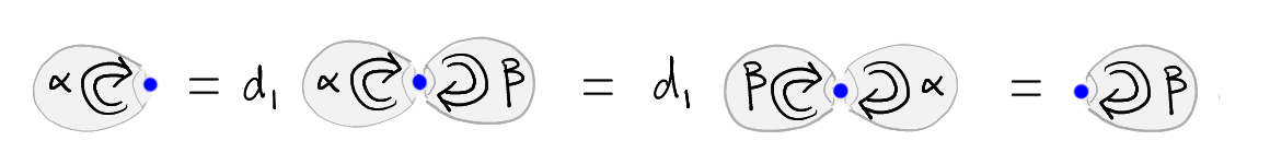
There is a more heuristic explanation underlying this undefinability result (see also here for details), which we illustrate in Figure 1. Namely, consider two \(2\)-cells \(\alpha\) and \(\beta\) each of whose domain and codomain is the identity on an object (indicated by a blue point in the Figure). Since the codomain of \(\alpha\) equals the domain of \(\beta\) we may compose \(\alpha\) with \(\beta\). Similarly, we may compose \(\beta\) with \(\alpha\). In a strict \(n\)-category these composites will be equal (by the “strict Eckmann-Hilton argument”). Now imagine a \(3\)-cells whose domain is the composite of \(\alpha\) with \(\beta\), and whose codomain is trivial (i.e. the double identity on the blue point). Then the operation of “taking the first face” of that \(3\)-cell is not well-defined (in the Figure, we indicate this operation by the symbol \(d_1\)): indeed, the “first face” may be either \(\alpha\) or \(\beta\). In other words, this \(3\)-cell doesn’t have well-defined face maps for either of its two boundary \(2\)-cells.

Figure 1. Since a wedge of 2-cells has a permuting symmetry (the strict Eckmann-Hilton argument), it yields an ill-defined boundary.

The role of degeneracies

A first root of the issue (as should be clear from Figure 1) is the presence of degenerate boundaries of cells. Simon Henry shows in [2] that computads without units form a presheaf category, and Amar Hadzihasanovic in [3] defines classes of computadic shapes “with spherical boundary” (which, in particular, cannot have degenerate domain or codomain) on which one can build models of higher categories. However, keeping the generality of the question intact and allowing for degeneracies of all types, will lead us on a quite different path to a resolution.

The role of strictness

A second, and ultimately deeper root of the issue is strictness (the strict version of the Eckmann-Hilton argument yields the central equality in Figure 1). As stated here, the failure of free strict higher categories to form a presheaf category may be abstractly resolved by working with free (appropriately) weak higher categories. However, this abstract observation has not given rise to a concrete combinatorial description of an underlying “category of cell shapes”, which is what we are chasing after here.

Aside: the role of directedness

Relatedly, one could consider undirected cells in higher groupoids in place of directed cells in higher categories (cells in categories are, of course, directed by designating a domain and a codomain part of their boundary). Once more, combinatorially describing “all shape” of undirected cells is difficult—in fact, even in a simplified case it is algorithmically impossible. Namely, we can consider undirected (i.e. ordinary) “regular cells”: a regular cell is a cell homeomorphic to a ball (and the same holds for each of its boundary cells). Since regular cells can have arbitrarily many cells in their boundary, there are infinitely many regular \(n\)-cells (starting in dimension \(n = 2\)), and so we might attempt to list at least those regular \(n\)-cells with less than \(k\) boundary cells. However, while this list must be finite, it cannot be produced for general \(k \in \mathbb{N}\). This roots in the computational obstruction that we cannot algorithmically recognize balls and spaces (explained further in [4]).

Defining “weak” computadic cells

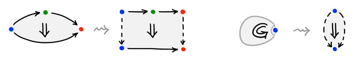
We will “weaken” the data of a computadic cell (we start with the heuristic idea, and latter comment on its formalization). Given a cell \(C\), with boundary \(\partial C\) decomposed into the cell’s “domain” \(\partial_- C\) and “codomain” \(\partial_+ C\) (each of which are similarly decomposed), the basic consistency condition for such inductive decompositions is given by the following equations (sometimes called “globularity condition”):

\[\partial_- \partial_- C = \partial_- \partial_+ C,\] \[\partial_+ \partial_- C = \partial_+ \partial_+ C.\]

Instead of structureless equalities, we want to consider these conditions as arrows themselves (turning equalities into arrows is a recurrent theme in category theory):

\[\partial_- \partial_- C \dashrightarrow \partial_- \partial_+ C,\] \[\partial_+ \partial_- C \dashrightarrow \partial_+ \partial_+ C.\]

The ramifications of this “structurification” are illustrated in Figure 2: where the globularity conditions of ordinary cells are turned into “structure” indicated by dashed arrows.

Figure 2. Ordinary cells turned into cells with globularity as structure.

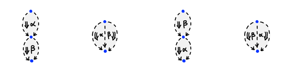
This change also affects composites of cells (i.e. pasting diagrams): namely, in the case of the problematic pasting diagram depicted in Figure 1, we now find four different pasting diagrams in its place, as shown in Figure 3.

Figure 3. Revisiting pasting diagrams of two cells with degenerate boundary, now with globularity as structure.

It will be useful to refer to such “structurified” cells by a name: we will call them framed computadic cells. We will give further reason for why one should consider framed computadic cells in a moment (and then also discuss how to formalize them). Let us, however, first record that the idea of framed computadic cells outlined above indeed solves the problem that we set out to solve.

Punchline. Framed computadic \((k+1)\)-cells can have any pasting \(k\)-diagram of framed computadic \(k\)-cells in their domain respectively codomain (including the empty one), and in this sense they form a “universal” class of computadic shapes as we set out to define. Moreover, presheafs on framed computadic cells yield (a notion of weak) computads.

Dual geometric interpretation

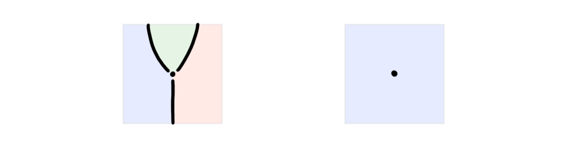
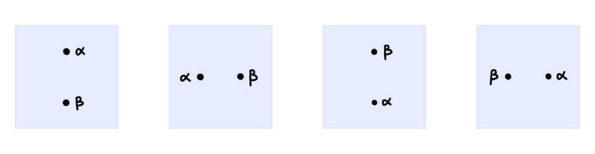
Framed computadic cells (and their pasting diagrams) can be understood in terms familiar to many readers by dualizing their geometry. (Roughly, “dualization” turns \(k\)-cells in a pasting \(n\)-diagrams into an \((n-k)\)-manifold in a so-called “manifold \(n\)-diagram” with the property that incidence relations are preserved: if cell \(C\) is a face of cell \(D\), then dual manifold \(C^\dagger\) contains dual manifold \(D^\dagger\) in its boundary.) For \(2\)-cells and pasting \(2\)-diagrams, this dualization yields familiar diagrams usually called “string diagrams”. For instance the two \(2\)-cells shown in Figure 2 dualize to the string diagrams shown in Figure 4.

Figure 4. Duals string diagrams of the framed \(2\)-cells in Figure 2.

Similarly, the four pasting diagrams shown earlier in Figure 3 dualize to the four string diagrams shown in Figure 5.

Figure 5. Duals string diagrams of the pasting \(2\)-diagrams in Figure 3.

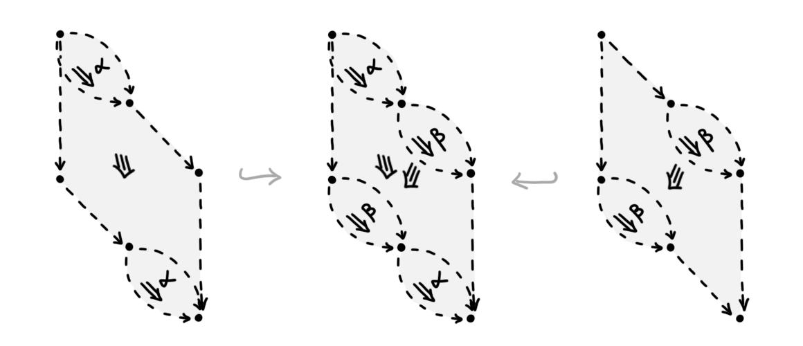
All four diagrams in Figure 5 are further related by manifold \(3\)-diagrams, namely, the so-called “braid” and its inverse. We illustrate the braid in Figure 6.

Figure 6. The braid as a manifold \(3\)-diagram.

Importantly, we can now “dualize” this manifold \(3\)-diagram to recover a pasting \(3\)-diagram of framed computadic cells, as shown in Figure 7. The pasting diagram consists of two 3-cells, as indicated by inclusions of each cell on the left and right of the diagram. (N.B: Note that both 3-cells are in fact degenerate cells: indeed, they are degeneracies of 2-cells. This reflects that their duals, the two “braid strands” in Figure 6, are manifolds of dimension \(1 = (3-2)\). Importantly, despite both 3-cells being degenerate individually, the pasting diagram itself cannot be expressed as a degeneracy of a simpler diagram.)

Figure 7. The pasting diagram of framed computadic cells dual to the braid.

We emphasize (as illustrated by the preceding examples) that the study of manifold \(n\)-diagrams of “framed manifolds” is fully equivalent to the study of pasting \(n\)-diagrams of framed computadic cells. However, the former perspective will be more familiar to most reader: indeed, the idea of “string diagrams”, “surface diagrams”, and in higher dimensions “manifold diagrams”, has been around for a long time! The difficulty has been the formalization of these diagrams in all dimensions—previous approaches worked their way only up to dimension 3 (and partially 4). This problem of a general formalization is solved by the combinatorial theory developed in [4] and [5]. Both references, as well as a note on manifold diagrams, contain more details on the matter.

Definition and framed regular cells

Framed computadic cells can be formally defined in two (fully equivalent) ways.

• Firstly, one can define manifold diagrams and then obtain framed computadic cell by dualizing “manifold diagram singularities”. This is further discussed in the note on manifold diagrams (and in [6]).

• Secondly, framed computadic cells can be obtain by endowing so-called “framed regular cells” with additional structure. The idea of framed regular cells is spelled out in [4] by following general principles for endowing classical objects from combinatorial topology with “framing structure”. There, it is also shown that framed regular cells have a concise combinatorial description as towers of “constructible combinatorial line bundles” and a large range of properties can be established on these grounds. Framed computadic cells can be obtained as “quotients” of framed regular cells, where quotients indicate which cells are degenerate (and enforce the globularity conditions).

Remark. We chose the terminology to indicate that the notion framed regular cells “precedes” the categorical context of the notion of framed computadic cells: framed regular cells “don’t care” about the distinction of domain and codomain, or the “globularity conditions” \(\partial_\pm \partial_- C \dashrightarrow \partial_\pm \partial_+ C\) in the way framed computadic cells do; in particular, globularity arrows may have more complicated structure than simply “fattened” identities.

References

[1] “Higher Operads, Higher Categories”, Leinster

[2] “Non-unital polygraphs form a presheaf category”, Henry

[3] “Diagrammatic sets and rewriting in weak higher categories”, Hadzihasanovic

[4] “Framed Combinatorial Topology”, Dorn + Douglas

[5] “Associative \(n\)-categories”, Dorn

[6] “Manifold diagrams and tame tangles”, In preparation, see here for updates