
From trusses to diagrammatic computads to combinatorial manifold diagrams
Abstract. This note gives a fast introduction to the rich combinatorial theory of trusses. We also discuss how presheafs of truss blocks give rise to diagrammatic computads, and how this can be used to understand manifold diagrams in purely combinatorial terms.
This note is part of a series.
UPDATE (Mar 2023). The vague term ‘weak computads’ was replaced by the much better term ‘diagrammatic computads’. Also several new articles appeared which contain introductory material about trusses.
Introduction
We give an overview of the basic combinatorial theory of trusses. The notion of “trusses” was introduced in [1], and extends the notion of “singular cubes” from [2] to a self-dual theory that combinatorially describes both “cell geometry” and “string geometry”. In particular, as discussed in [1], trusses provide a computable foundation for framed combinatorial topology which deals with spaces that are built from “framed” cells (the resulting notion of framed space can, for instance, be thought of as a geometric model for higher categorical structures). In this note, we will focus mainly on the combinatorics and less on the geometry. Our main aim, firstly, is to give the core combinatorial definitions in the theory of trusses. Secondly, we will sketch how to bridge the theory of trusses with classical ideas in higher categories by introducing a notion of “diagrammatic computad”, which will lead us to formally rediscover “computadic pasting diagrams” and, dually, “manifold diagrams”—both notions were discussed already in earlier notes.
Trusses are “towers of combinatorial constructible bundles”. Fibers of these bundles are “1-dimensional trusses”, usually referred to as “1-trusses”. Conversely, trusses are referred to as “\(n\)-trusses” are given by a tower of \(n\) bundles of \(1\)-trusses (ending in the \(0\)-truss, the “point”). There are many interesting aspects to the theory of trusses, and we shall introduce notions of “bundles”, “maps”, and “duals” for them; centrally. As we will see, similar to other combinatorial shapes (such as simplices, cubes, opetopes, etc.), maps include “faces” and “degeneracies”—importantly, we will also be able to combinatorially represent the dual notions of maps, namely notions of “embeddings” and “subdivisions”. The natural starting point for this discussion is dimension \(1\), which we will discuss first before introducing trusses in dimension \(n\).
1-Trusses
1-Trusses are the entrance path posets of (tangentially) framed stratified manifolds of dimension \(0\) or \(1\)—these stratifications are called 1-meshes.
Definition (1-Meshes; see [1], Ch. 4). A 1-mesh \((M,f,\gamma)\) is a connected \(k\)-manifold, \(k \in \{0,1\}\), together with a stratification \(f\) of \(M\) whose strata are open disks, as well as a tangential framing \(\gamma\) of \(M\). \(\blacklozenge\)
Note that a framing of a connected \(0\)-dimensional manifold is trivial. A framing of a connected \(1\)-dimensional manifold is equivalently an orientation (in particular, up to equivalence, there are exactly two framings).
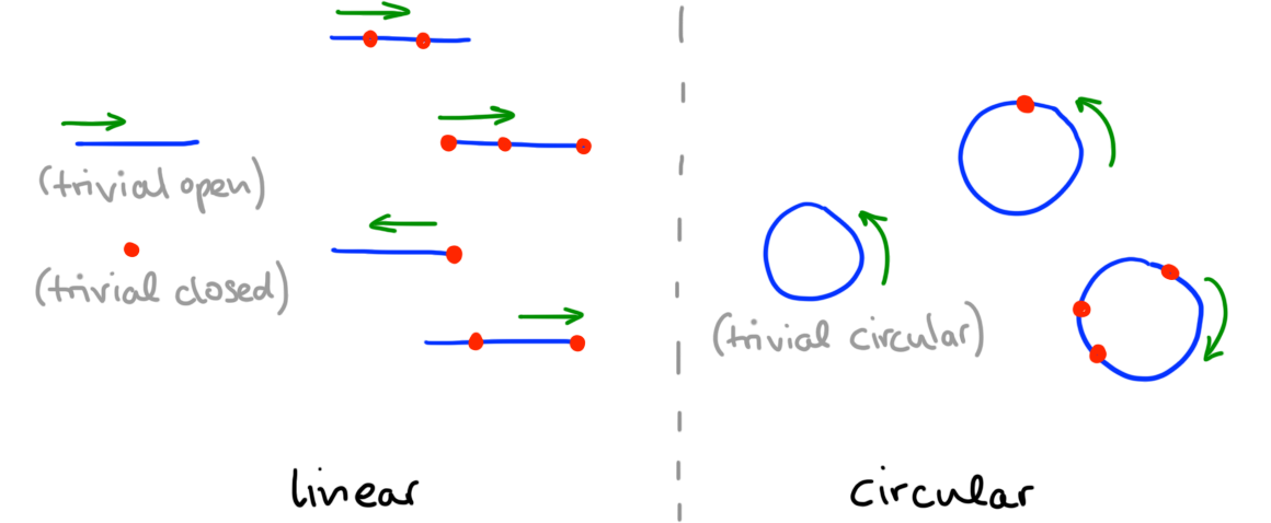
Terminology (Linear and circular 1-meshes). A \(1\)-mesh \((M,f,\gamma)\) is called linear if \(M\) is contractible, and circular otherwise. \(\blacklozenge\)
Example (1-Meshes) In Figure 1 we illustrate 1-meshes (both linear and circular ones). 0-disk strata are highlighted in red, 1-disk strata in blue. Framings are indicated by green arrows. \(\blacklozenge\)
1-Trusses are the combinatorial counterparts of 1-meshes, obtained by passing to their entrance path posets together with combinatorial data representing disk dimensions and the framing. (Recall from a previous note that entrance path posets of stratifications are posets whose objects are strata and whose arrows indicate when one stratum borders on another.) Like 1-meshes, 1-trusses come both in “linear” and “circular” flavors. For simplicity we will only consider the linear case here—therefore, henceforth “1-mesh” will mean “linear 1-mesh” and similarly, the reader can think of “1-truss” as referring to “linear 1-truss” (as opposed to a notion of “circular 1-truss”, which we will not define here).
Definition (1-Trusses; see [1], Ch. 2). A 1-truss \((T,\leq, \dim, \fleq)\) is a poset \((T,\leq)\) together with a poset map \(\dim : (T,\leq) \to [1]\op\) (where \([1]\op\) is the poset \(1 \to 0\)), as well as a total order \((T,\fleq)\), satisfying the following: there exist a 1-mesh \((\abs{T},f,\gamma)\) that admits
- an isomorphism \(\phi : (T,\leq) \iso \Entr(f)\),
- with \(\dim(s) = \dim(\phi(s))\) for all \(s \in T\),
- and \(s \fleq t\) if and only if there is an oriented path starting in the stratum \(\phi(s)\) and ending in \(\phi(t)\). \(\blacklozenge\)
In the preceding definition, the 1-mesh \((\abs{T},f,\gamma)\) is called a geometric realization of the 1-truss \((T,\leq, \dim, \fleq)\). Note, for fixed geometric realization, the choice of isomorphisms \(\phi\) is necessarily unique in the previous definition (and the choice of geometric realization is itself unique up to contractible choice; we will come back to this point later).
Example (1-Trusses). In Figure 2 we illustrate 1-trusses \((T,\leq,\dim,\fleq)\); the order \(\leq\) is indicated by arrows between objects; the map \(\dim\) is indicated by coloring the objects \(s\) in red if \(\dim(s) = 0\) and in blue if \(\dim(s) = 1\); the linear order \(\fleq\) is indicated by arranging objects on a line together with a direction given by a (green) “coordinate axis” arrow. \(\blacklozenge\)
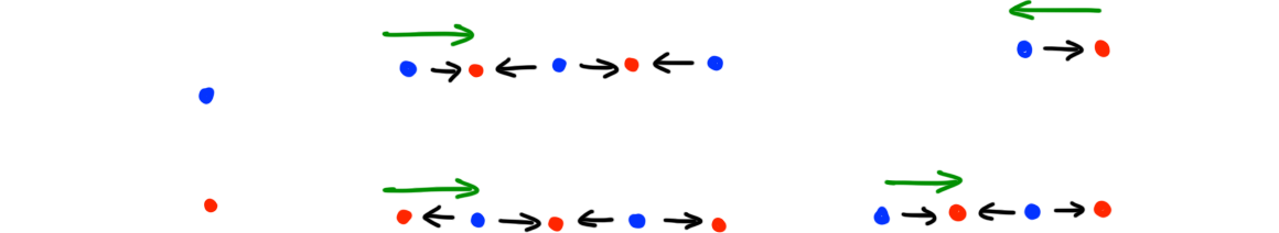
Terminology (Basic 1-truss terms). Given a 1-truss \((T,\leq,\dim,\fleq)\) we call \(\leq\) the face order, \(\dim\) the dimension map, \(\fleq\) the frame order. We say \(s \in T\) is a singular element if \(\dim(s) = 1\), and a regular element otherwise. The subsets of singular resp. regular objects of \(T\) will be written as \(T_0\) resp. \(T_1\) (note: in [1] these are written as \(\mathrm{sing(T)}\) resp. \(\mathrm{reg}(T)\)). A 1-truss is called closed if its geometric realization is compact (as a space). A 1-truss called open if its geometric realization is an open interval (as a space). \(\blacklozenge\)
In the next sections we will discuss three central aspects of 1-truss theory: (1), they behave well in families, (2), they admit several types of maps with concrete geometric interpretation (going beyond traditional “face” and “degeneracy” maps), and (3), they can be combinatorially dualized, which again has concrete geometric interpretation. We will discuss (1), (2), and (3) in order.
Bundles
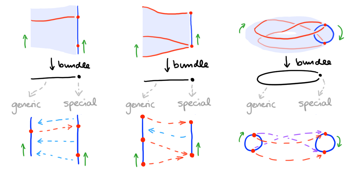
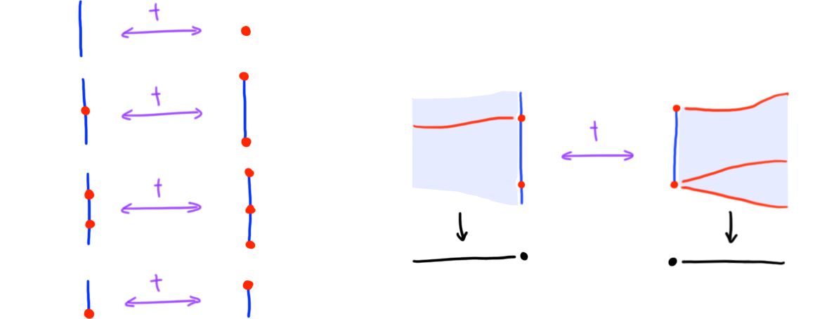
Considering 1-truss in families gives rise to “bundles of 1-trusses”. Just as 1-trusses are combinatorial models of 1-meshes, “1-truss bundles” are combinatorial models of “1-mesh bundles”. To motivate our definitions, let us therefore start by illustrating the desired notion of bundles geometricbally. Recall that “stratified bundles” are fiber bundles of stratified spaces \(p : (M,f) \to (B,g)\) admitting local trivialization over each base stratum. We will consider stratified bundles in which each fiber \(p\inv(b)\) has the structure of a 1-mesh. Crucially, in a 1-mesh bundle we want transition maps of fibers in these bundles to preserve the data of a 1-mesh: this means, firstly, that we need to preserve framings when passing between fibers (in other words, the orientations of fibers locally point in the “same direction”); secondly, we want to preserve dimensions of strata appropriately, in that \(0\)-dimensional strata in the generic fiber must “transition to” \(0\)-dimensional strata in the special fiber, while dually, \(1\)-dimensional strata in the special fiber must “be transitioned into” from \(1\)-dimensional strata in the generic fiber.
Example (1-Mesh bundles). The resulting types of bundles are illustrated in Figure 3: underneath each bundle, we illustrate the bundle generic and special fiber, together with an indication of functional relations (dotted arrows) that indicate how \(0\)-strata “transition-to” other \(0\)-strata (red/purple arrows), and how to \(1\)-strata we “transition-from” other \(1\)-strata (blue arrows). (Note in the last example, we omit blue “transition-from” arrows for simplicity). \(\blacklozenge\)
In general, the base of such 1-mesh bundles may be any stratified space \((B,g)\)—combinatorially, we will slightly simplify our life, and work with a base poset \((B,\leq)\) in its place (note, while stratifications generally cannot be recovered from their entrance path posets, they can be recovered if strata are “regular cells”; and this is the case we are ultimately interested in).
Phrasing the two core properties of fiber transitions in 1-mesh bundles (namely, “frame” and “dimension” preservation) observed above in combinatorial terms, we are now led to the following definition of 1-truss bundles.
Definition (1-Truss bundles). A 1-truss bundle
\[p : (T,\leq,\dim,\fleq) \to (B,\leq)\]consists of a poset map \(p : (T,\leq) \to (B,\leq)\), another poset map \(\dim : (T,\leq) \to [1]\op\), and a fiberwise total order \((p\inv(x),\fleq)\) (for each \(x \in B\)) such that the following holds.
- For each object \(x\) in \(B\), the datum \((p\inv(x),\leq,\dim,\fleq)\) (with \(\leq\) and \(\dim\) restricted to the fiber \(p\inv(x)\)) is a 1-truss.
- For each morphism \(x \to y\) in \(B\), \(p\inv(x \to y)\) is a valid fiber transition, meaning that the relation \(R(a,b) \iff a \to b\) (where \(a \in p\inv(x)\) and \(b \in p\inv(y)\)) satifies the following:
- Frame preservation (called “bimonotocity” in [1]). If \(a \fles a'\), \(R(a,b)\) and \(R(a',b')\) then \(b \fleq b'\). Dually, if \(b \fles b'\), \(R(a,b)\) and \(R(a',b')\) then \(a \fleq a'\).
- Dimension preservation (called “bifunctionality” in [1]). There exists a “transition-to” function \(R_0 : p\inv(x)_0 \to p\inv(y)_0\) such that, for \(a \in p\inv(x)_0, b \in p\inv(x)_0\) we have \(R(a,b) \iff R_0(a) = b\). Dually, there exists a “transition-from” function \(R_1 : p\inv(y)_1 \to p\inv(x)_1\) such that, for \(a \in p\inv(x)_1, b \in p\inv(x)_1\) we have \(R(a,b) \iff a = R_1(b)\). \(\blacklozenge\)
If we were to spell out our definition of 1-mesh bundles further (which is done in [1]) we would find that 1-mesh bundles up to an appropriate notion of equivalence (and over sufficiently regular base) are exactly 1-truss bundles up to an appropriate notion of structure-preserving isomorphism. This provides, if you want, a geometric-semantic correctness result for the above definition. We will return to this comparison later in the context of \(n\)-trusses (and their geometric realization as \(n\)-meshes).
Note that 1-trusses \((T,\leq,\dim,\fleq)\) are exactly 1-truss bundles over the terminal poset \([0] = \{0\}\).
Notation (Keeping truss [bundle] data implicit). We usually keep much of the data of a 1-truss bundle implicit and simply write \(n\)-truss bundles as maps \(p : T \to B\). The simplfication similarly applies to 1-trusses where we write \(T\) in place of \((T,\leq,\dim,\fleq)\); analogously, we usually write 1-meshes simply as \(M\) and 1-mesh bundles as \(M \to B\). \(\blacklozenge\)
Construction (Bordisms and classification of bundles). Given trusses \(T\) and \(S\), a 1-truss bordism \(R : T \proto S\) is a 1-truss bundle \(p : R \to [1]\) over the interval poset \([1] = \{0 \to 1\}\), whose first fiber is \(p\inv(0) = T\) and whose second fiber is \(p\inv(1) = S\). In [1] we give a more direct definition of 1-truss bordisms (and, in fact, define bundles in terms of bordisms and not the other way around) for the following reason: 1-truss bordisms are the arrows of a category of 1-truss bordisms \(\ttr 1\). Each truss bundle \(p : T \to B\) has a classifying functor \(\fcl {} p : B \to \ttr 1\), which maps objects \(x \in B\) to the fiber truss \(p\inv(x)\), and arrows \((x \to y)\) to the fiber bordism \(p\inv(x \to y)\) (or more precisely, to the pullback 1-truss bundle of \(p\) along the map \([1] \iso (x \to y) \to B\)). 1-Truss bundles over \(B\) up to equivalence (equivalences are defined in the next section) are in correspondence with functors \(B \to \ttr 1\) up to natural isomorphism. \(\blacklozenge\)
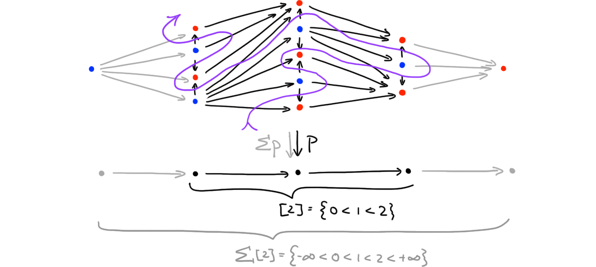
Remark (Truss induction). One aspect of the theory of 1-truss bundles which we do properly not touch upon is “truss induction” (thorougly discussed in [1], Section 2.2); this proves that “\((n+1)\)-simplices in 1-truss bundles over \(n\)-simplices are linearly ordered”. Here, we will only provide a visual cue. Any truss bundle \(p : T \to [n]\) has a suspension \(\Sigma p : \Sigma T \to \Sigma [n]\) obtained by adjoining new initial and terminal elements to \(T\) resp. \([n]\) (require the initial element to have dimension \(1\) and the terminal element dimension \(0\)). The restriction of \(\Sigma p\) to the spine of \(\Sigma [n]\) gives a projection of graphs that can be visualized in a plane (see the example in Figure 4). There is a unique path such that: the path passes through all arrows in the fibers of the projection; in between any two such passages (and before/after the first/last such passage) it passes through exactly one other arrow; this arrow runs between a dim-1 and dim-0 object. We illustrate the path in Figure 4. This path encodes a linear order of \((n+1)\)-simplices in \(T\)—inducting along this path is a useful technique when dealing with truss bundles, and we refer to this technique as truss induction. \(\blacklozenge\)
Maps
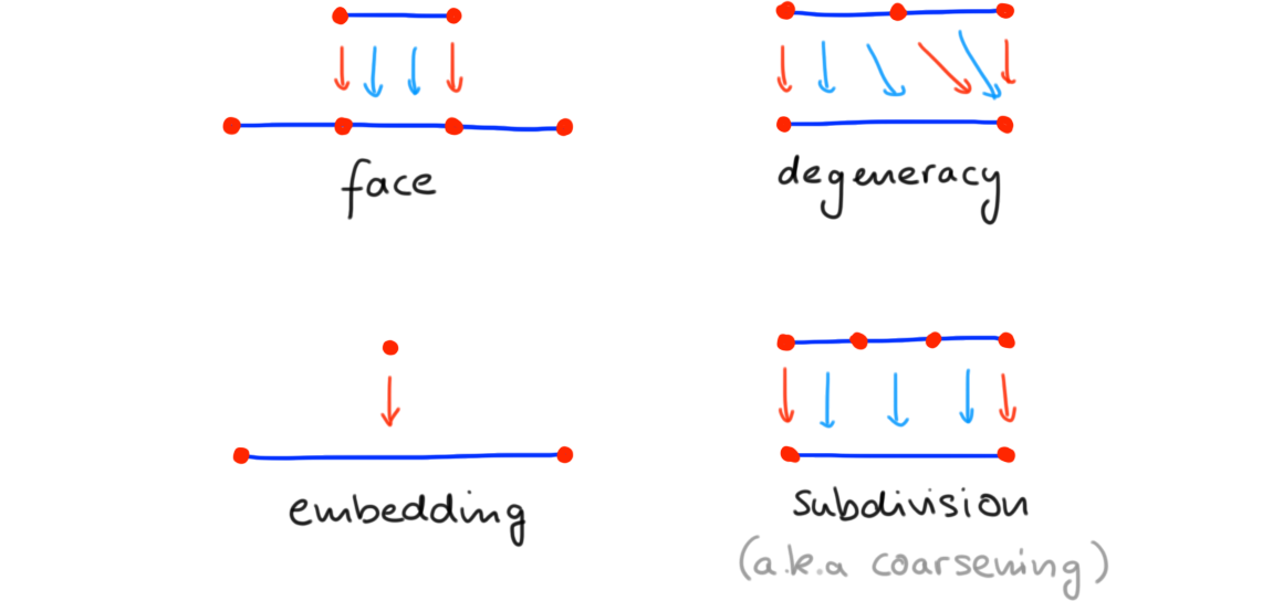
We next discuss maps of 1-trusses. In the previous section, we saw that bordisms of 1-trusses are combinatorial models of fiber transitions in bundles of 1-meshes. In contrast, maps of 1-trusses are combinatorial models of “maps of 1-meshes”—the latter notion does the obvious: a map of 1-meshes is a stratified map which preserve the framings (in other words, they are orientation-preserving). Several such maps of 1-meshes are shown in Figure 5. Importantly, depending on how such maps interact with strata dimension they may be further distinguish (examples are given in Figure 5).
- A 1-mesh map that maps \(0\)-strata to \(0\)-strata is called a singular map. Further, it is called
- a face map (or \(\mathbf{F}\)-map) if it is injective on strata,
- a degeneracy (or \(\mathbf{D}\)-map) map if is surjective on strata.
- A 1-mesh map that maps \(1\)-strata to \(1\)-strata is called a regular map. Further, it is called
- an embedding (or \(\mathbf{E}\)-map) if it is injective on strata.
- a coarsening (or \(\mathbf{C}\)-map) if it is surjective on strata.
- A map that is both regular and singular is called balanced. A balanced 1-mesh map that is bijective on strata is called a 1-mesh equivalence (it is, up to homotopy, a stratified homeomorphism).
Note coarsenings are sometimes called “subdivisions” or “refinements”.
Example (1-mesh maps). We illustrate 1-mesh maps in Figure 5; note that we illustrate all map types in the case of closed linear 1-meshes (the classification of course equally applies to other mesh types). \(\blacklozenge\)
Note that we may also refer to coarsenings as both subdivisions or refinements (often as a description of the “opposite” process of coarsening).
Let us now translate these notions of maps into the setting of 1-trusses.
Definition (1-Truss maps) Given \(1\)-trusses \(T\) and \(S\), a 1-truss map \(F : T \to S\) is a map that preserves both face orders \(F : (T,\leq) \to (S,\leq)\) and frame orders \(F : (T,\leq) \to (S,\leq)\). \(\blacklozenge\)
We saw that every 1-truss \(T\) is geometrically realized by an 1-mesh \(\abs{T}\) (uniquely so up to 1-mesh isomorphism) such that \(\Entr \abs{T} = T\). Similarly, 1-truss maps have geometric realizations: we say that a 1-mesh map \(\abs{F} : \abs{T} \to \abs{S}\) geometrically realizes the 1-truss map \(F : T \to S\) if \(\Entr \abs{F} = F\). Geometric realization of 1-truss maps are unique up to contractible choice in the space of realizations.
Terminology (Map types). A 1-truss map \(F : T \to S\) is called a \(\bC/\bD/\bE/\bF\)-map if its realization is an \(\bC/\bD/\bE/\bF\)-map of 1-meshes. Similarly one defines 1-truss maps that are singular, regular, balanced and equivalences. \(\blacklozenge\)
The notion of maps of 1-truss is easily generalized to the case of 1-truss bundles.
Definition (Truss bundle maps). Given 1-truss bundles \(p : T \to B\) and \(q : S \to C\) a bundle map \(F : p \to q\) is a poset map \(F : T \to S\) commuting with \(p\) and \(q\) by a square
\[\begin{CD} T @>{F}>> S\\ @VpVV @VVqV \\ B @>>> C \end{CD}\]such that \(F\) restricts to a 1-truss map on each fiber. We say \(F\) is a \(\bC/\bD/\bE/\bF\)-map (resp. singular, regular, balanced or an equivalence) if it is so fiberwise. \(\blacklozenge\)
Notation (Categories of trusses and truss bundles). Let’s denote the category of 1-trusses and their maps by \(\truss 1\), and the category of 1-truss bundles and their maps by \(\trussbun 1\).
Dualization
Let us turn to a final important aspect of 1-truss theory: the combinatorial phrasing of (Poincaré) duality. Geometrically, dualization does the following: given a 1-mesh \(M\), its dual \(M^\dagger\) is the 1-mesh in which \(0\)-strata and \(1\)-strata of \(M\) are turned into \(1\)-strata resp. \(0\)-strata without affecting the direction of the framing—we illustrate this in Figure 6 (we also show how the idea applies to 1-mesh bundles).
Formally, and combinatorially, this is defined as follows.
Definition (Dualization of 1-trusses, bundles, bordisms and maps) Given a 1-truss \(T \equiv (T,\leq,\dim,\fleq)\) its dual truss \(T^\dagger\) is the 1-truss \((T,\leq\op,\dim\op,\fleq)\) (where \(\dim\op : (T,\leq\op) \to ([1]\op)\op \iso [1]\op\)).
Similarly, given a 1-truss bundle \(p : (T,\leq,\dim,\fleq) \to B\), its dual bundle \(p^\dagger\) is the bundle \(p : (T,\leq\op,\dim\op,\fleq) \to (B,\leq\op)\). In particular, given a 1-truss bordism \(R : T \proto S\), its dual bordism is the 1-truss bordism \(R^\dagger : S \proto T\) such that \(R(a,b) \iff R^\dagger(b,a)\).
Given a 1-truss bundle map \(F : T \to S\), its dual map \(F^\dagger\) is the map \(F : T^\dagger \to S^\dagger\) (i.e. identical to \(F\) on objects). \(\blacklozenge\)
Earlier, we introduced the categories \(\ttr 1\), \(\truss 1\) and \(\trussbun 1\); dualization acts as follows on these categories.
Observation (Dualization on categories). Dualization of 1-trusses and their bordisms yields an isomorphism of categories
\[\dagger : \ttr 1 \iso (\ttr 1)\op : \dagger\]Dualization of 1-truss (bundles) and their maps yields isomorphisms
\[\begin{aligned} \dagger : \truss 1 &\iso \truss 1 : \dagger \\ \dagger : \trussbun 1 &\iso \trussbun 1 : \dagger \end{aligned}\]The functor \(\dagger\) further maps
- \(\bF\)-maps to \(\bE\)-maps and vice versa,
- \(\bD\)-maps to \(\bC\)-maps and vice versa. \(\blacklozenge\)
Let us further distinguish two important subcategoeries in the above categories.
Remark (Open and closed 1-trusses). Note that \(\dagger\) sends closed 1-trusses to open 1-trusses and vice versa. \(\blacklozenge\)
Labels and stratifications
Labels
Given a topological space \(X\), and a categorical structure \(\iC\) (e.g. a poset, category, or higher category) a “labeling” of \(X\) is a functor \(\Pi_\infty X \to \iC\) from the fundamental (\(\infty\)-)groupoid of \(X\) into \(\iC\). In the case of stratified topological spaces, this generalizes to a functor from the fundamental \(\infty\)-category (whose morphisms are not mere paths but entrance paths) into \(\iC\). If we work with sufficiently simple stratifications (which we ultimately do), this fundamental \(\infty\)-category becomes equivalent to the stratification’s entrance path poset. As we’ve seen, in the case of 1-meshes (resp. their bundles) entrance path posets are modeled by the corresponding 1-trusses (resp. their bundles). This motivates the following definition.
Definition (Labeled 1-trusses and bundles). Let \(\iC\) be a (ordinary) category. A \(\iC\)-labeled 1-truss \(T \equiv (\und T, \lbl_T)\) consists of an ‘underlying’ 1-truss \(\und T \equiv (\und T,\leq,\dim,\fleq)\) together with a ‘labeling’ functor \(\lbl_T : (\und T,\leq) \to \iC\). Similarly, a \(\iC\)-labeled 1-truss bundle \(p \equiv (\und p, \lbl_p)\) consists of an ‘underlying’ 1-truss bundle \(\und p : (T,\leq,\dim,\fleq) \to B\) together with a ‘labeling’ functor \(\lbl_p : (T,\leq) \to \iC\). \(\blacklozenge\)
Definition (Maps of labeled 1-trusses and bundles). Given two labeled 1-truss bundles \(p \equiv (\und p : T \to B, \lbl_p : T \to \iC)\) and \(q \equiv (\und q : S \to C, \lbl_q : S \to \iC)\), a labeled bundle map \(F : p \to q\) is a map \(\und F : \und p \to \und q\) of underlying bundles together with a functor \(\lbl_F : \iC \to \iD\) of labels such that the following commutes
\[\begin{CD} \iC @<{\lbl_p}<< T @>{\und p}>> B \\ @V{\lbl_F}VV @VVFV @VVV \\ \iD @<{\lbl_q}<< S @>{\und q}>> C \end{CD}\]The definition specializes to a notion of labeled 1-truss maps if we set \(B = C = [0]\). (One may also weaken the definition, by allowing the left square in the above diagram to commute up to natural (iso)morphism). \(\blacklozenge\)
The central observation about \(\iC\)-labeled 1-truss bundles is that they have a classifying category; this is the category of \(\iC\)-labeled 1-truss and their bordisms.
Construction (Labeled bordisms and classification of labeled bundles) A \(\iC\)-labeled 1-truss bordism \(R : T \proto S\) is a labeled 1-truss bundle \((\und R : U \to B, \lbl_R : U \to \iC)\) with base equal to the interval poset \(B = [1]\); its domain \(T\) is the \(\iC\)-labeled 1-truss obtain by restricting \(\und R\) to \(\{0\} \into [1]\) and accordingly restricting \(\lbl_R\), its codomain \(S\) is similarly obtain by restriction to \(\{1\} \into [1]\). Importantly, \(\iC\)-labeled 1-truss bordisms compose: given \(\iC\)-labeled 1-truss bordisms \(R : T \proto S\), and \(Q : S \proto U\), then there exists a unique labeled 1-truss bordism \(P : T \proto U\) such that \(P,Q,R\) are the restrictions of a single \(\iC\)-labeled 1-truss bundle over the 2-simplex \([2]\) (to the arrows \((0 \to 2)\), \((1 \to 2)\) resp. \((0 \to 1)\)). We set \(P \equiv R \circ Q\). The proof of this construction uses truss induction over the 2-simplex (as we will briefly revisit later on, there are also \(\infty\)-categorical generalizations, which then use truss induction in its full power over general \(n\)-simplices).
As a result, we obtain the category of \(\iC\)-labeled 1-truss bordisms \(\lttr 1 \iC\), whose objects are \(\iC\)-labeled 1-trusses and whose morphisms are \(\iC\)-labeled 1-truss bordisms. Each \(\iC\)-labeled truss bundle \(p \equiv (\und p : T \to B, \lbl_p : T \to \iC)\) has again a classifying functor \(\fcl {} p : B \to \lttr 1 \iC\): this maps objects \(x \in B\) to the \(\iC\)-labeled fiber truss \((\und p\inv(x), \lbl_p : \und p\inv(x) \to \iC)\), and arrows \((x \to y)\) to the \(\iC\)-labeled fiber bordism \((\und p\inv(x \to y),\lbl_p : \und p\inv(x \to y) \to \iC)\). This yields a correspondence of \(\iC\)-labeled 1-truss bundles over \(B\) with functors \(B \to \lttr 1 \iC\) (up to appropriate notions of equivalences). \(\blacklozenge\)
As an aside, for the category theorists among us it could be fun to think about the following observation.
Remark (Labeled truss bordisms as a vertical comma category). There is an embedding \(\ttr 1 \into \mathrm{Prof}\) of the category of 1-truss bordisms into the bicategory of profunctors, which regards 1-truss bordisms as \(\Bool\)-enriched profunctors and post-composes them with the inclusion \(\Bool \into \SetCat\) (the fact that this works is non-trivial; for instance relations \(\mathrm{Rel}\) do not (non-laxly) embed into profunctors \(\mathrm{Prof}\)). Using this embedding, a \(\iC\)-labeled 1-truss bordism is then exactly a square
\[\begin{array}{ccc} \und T & \xrightarrow{\quad \raisebox{.3ex}{$\scriptstyle \und R$} \quad}\mkern{-4.5ex}{\raisebox{.3ex}{$\tiny\vert$}}\mkern{4.2ex} & \und S\\\ \kern-3ex\raisebox{.3ex}{\rlap{$\scriptstyle \lbl_T$}}\kern+3ex\bigg\downarrow & \quad \Darr {\scriptstyle \lbl_R} & \bigg\downarrow\raisebox{.5ex}{\rlap{$\scriptstyle \lbl_S$}} \\\ \iC & \xrightarrow{\kern{.4em} \raisebox{.3ex}{$\scriptstyle \Hom_\iC$} \kern{.4em}}\mkern{-4.5ex}{\raisebox{.3ex}{$\tiny\vert$}}\mkern{4.2ex} & \iC \end{array}\]in the (pseudo) double category of profunctors \(\mathbb{P}\mathrm{rof}\). One can therefore think of \(\lttr 1 \iC\) as a “vertical comma category” of the horizontal embedding \(\ttr 1 \into \mathrm{Prof} \into \mathbb{P}\mathrm{rof}\) over \(\iC\). \(\blacklozenge\)
Stratifications
The “base case” of interest to us are labeling functors that are characteristic maps of stratifications. Recall that finite stratifications \((X,f)\) have (and are determined by their) continous characteristic maps \(f : X \to \Entr(f)\). Topologizing posets using the downward closed topology, this similar applies to posets: a (finitely) stratified poset \((P,f)\) determines and is determined by its characteristic map \(f : P \to \Entr(f)\)—the latter now is a poset map with the property that preimages \(f\inv(s)\) are non-empty connected subposets of \(P\) such that \(s \to r\) in \(\Entr(f)\) if and only if the upwards closure of \(f\inv(s)\) non-trivially intersects \(f\inv(r)\) in \(P\) (in [1], Appendix B, such maps are also called “connected-quotient” maps of posets).
Definition (Stratified 1-truss bundle). A stratified 1-truss bundle is a labeled 1-truss bundle in which the labeling functor is the characteristic map of a stratification. (The definition specializes to a notion of stratified 1-trusses if the base is trivial). \(\blacklozenge\)
Every poset labeled 1-truss bundle determines a stratified 1-truss bundle as the following construction shows.
Construction (Connected component splitting). Let \(P\) be a poset, and consider a \(P\)-labeled 1-truss bundle \(p \equiv (\und p : T \to B, \lbl_p : T \to P)\). There exists a unique factorization of the labeling by maps \(\mathrm{cc}(p) : T \to \Entr(p)\) and \(\mathrm{dd} : \Entr(p) \to P\) such that \(\mathrm{cc}(p)\) is the characteristic map of a stratification, and \(\mathrm{dd}(p)\) is a poset map with discrete preimages (this factorization has several universal properties, see [1], Appendix B). We can thus associate a stratified 1-truss bundle \((\und p, \mathrm{cc}(p))\) to \(p\), which is called the connected component splitting of \(p\). Usually, when referring to stratifications in the context of poset-labeled bundles we implicitly pass to their connected component splittings. \(\blacklozenge\)
The idea of “connected component splitting” bridges our variation of the notion of stratification with, for instance, the notion introduced in [3]: Lurie introduces “\(P\)-stratifications” as spaces \(X\) endowed with a continuous map \(f : X \to P\) to a poset \(P\). In the case of locally finite stratifications, this map splits uniquely by maps \(X \to \Entr(f) \to P\) in which the first map is a continuous characteristic map and the second map is a map with discrete preimages.
\(n\)-Trusses
We are finally ready to generalize our discussion to higher dimension. The process is straight-forward and has the following analog. The interval \(\bI\) is a 1-dimensional manifold. The total space of an \(\bI\)-fiber bundle over \(\bI\) is a 2-dimensional manifold—in fact, it homeomorphic to the square \(\bI^2 = \bI \times \bI\). By iteratively considering \(\bI\)-bundles over (the total space) of \(\bI\)-bundles we can build the \(n\)-cube \(\bI^n\). Replacing \(\bI\)-bundles by 1-truss bundles, this idea can be directly applied to define \(n\)-trusses. (Note also that the interval \(\bI\) is an \(\bI\)-bundle over the point \(\ast\) and, while this doesn’t add any information, we usually add this “terminal” bundle to all towers of bundles below.)
Definition (\(n\)-Trusses). An \(n\)-truss is a tower of 1-truss bundles \(p_i\)
\[T_n \xto {p_n} T_{n-1} \xto {p_{n-1}} T_{n-2} \to \cdots \to T_2 \xto {p_2} T_1 \xto {p_1} T_0 = [0]\]where the total poset \((T_i,\leq)\) of \(p_i\) is the base poset of \(p_{i+1}\). \(\blacklozenge\)
Bundles
The above definition immediately generalizes to a notion of “\(n\)-truss bundles” by omitting the condition \(T_0 = [0]\) and instead allowing \(T_0\) to be an arbitrary (finite) poset. However, let us be more general and also allow these bundles to be labeled.
Definition (Labeled \(n\)-truss bundles). For a category \(\iC\) and a poset \(B\), a \(\iC\)-labeled \(n\)-truss bundle \(p\) is a diagram of the form
\[\iC \xot{\lbl_p} T_n \xto {p_n} T_{n-1} \xto {p_{n-1}} \dots \xto {p_2} T_1 \xto {p_1} T_0 = B\]where the left most ‘labeling functor’ \(\lbl_p\) is a functor \((T_n,\leq \to \iC)\), while the remaining tower to its right consists of 1-truss bundles \(p_i\) which together form the ‘underlying \(n\)-truss bundle’ \(\und p\) of \(p\). \(\blacklozenge\)
Construction (Classification of \(n\)-truss bundles). A \(\iC\)-labeled \(n\)-truss bordism \(R : T \proto S\) is a \(\iC\)-labeled \(n\)-truss bundle over \([1]\), which restricts to (the \(\iC\)-labeled \(n\)-truss) \(T\) over \(\{0\} \into [1]\) and to \(S\) over \(\{1\} \into [1]\). As in the case \(n = 1\), such bordisms compose: given \(\iC\)-labeled \(n\)-truss bordisms \(R : T \proto S\), and \(Q : S \proto U\), then there exists a unique labeled 1-truss bordism \(P : T \proto U\) such that \(P,Q,R\) are the restrictions of a single \(\iC\)-labeled 1-truss bundle over the 2-simplex \([2]\) (to the arrows \((0 \to 2)\), \((1 \to 2)\) resp. \((0 \to 1)\)). We set \(P = R \circ Q\), and obtain the category of \(\iC\)-labeled \(n\)-truss bordisms \(\lttr n \iC\).
This category can be constructed in a more explicit, inductive manner (which also shows that \(\lttr n \iC\) exactly classifies \(\iC\)-labeled \(n\)-truss bundles). Consider, in the following diagram, the upper row of 1-truss bundles \(p_i\) together with the \(\iC\)-labeling \(\lbl_p\): this defines a \(\iC\)-labeled \(n\)-truss bundles \(p\).
\[\scriptsize \begin{CD} T_n @>{p_{n}}>> T_{n-1} @>{p_{n-1}}>> T_{n-1} @>{p_{n-2}}>> {\quad \cdots \quad} @>{p_2}>> T_1 @>{p_1}>> T_0 \\ @V{\lbl_p}VV @VVV @VVV @. @VVV @VVV \\ \iC @. {\lttr 1 \iC} @. {\lttr 1 {\lttr 1 \iC}} @. {\cdots} @. {\lttr {n-1} \iC} @. {\lttr n \iC} \end{CD}\]Just considering the top-bundle \(p_n\) together with the labeling \(\lbl_p\) we obtain a \(\iC\)-labeled 1-truss bundle \((p_n,\lbl_p)\); as we’ve seen such labeled bundles are classified by functors from the base of \(p_n\) (namely \(T_{n-1}\)) to \(\lttr 1 \iC\). But this classifying functor \(T_{n-1} \to \lttr 1 \iC\) now provides a labeling for the bundle \(p_{n-1}\); the resulting labeled 1-truss bundle is classified by a functor \(T_{n-2} \to \lttr 1 {\lttr 1 \iC}\). Inductively continuing this process, and setting
\[\lttr k \iC = \lttr 1 {\lttr {k-1} \iC}\]we eventually construct the functor \(T_0 \to \lttr n \iC\) as shown in the diagram–this functor “classifies” the labeled \(n\)-truss bundle \(p\). The seeming notational conflict (we’ve now doubly defined \(\lttr n \iC\)) is resolved by observing that both of our definitions are equivalent. Note further that the construction is functorial in \(\iC\) (exercise!): we thus obtain functors \(\ttr n : \mathrm{Cat} \to \mathrm{Cat}\), \(n \in \lN\), on the category of categories, and this is the \(n\)-fold iteration of the functor \(\ttr 1\).
(A more direct view on the classifying functor \(T_0 \to \lttr n \iC\) is the following: objects \(x\) in \(B\) are mapped to the labeled fiber truss over \(x\) in \(p\); morphisms \((x \to y)\) in \(B\) are mapped to the labeled fiber truss bordism over \((x \to y)\) in \(p\).) \(\blacklozenge\)
Remark (The quasicategory of labeled \(n\)-truss bordisms). Given a quasicategory \(\mathcal{C}\) we can form a simplicial set \(\lttr n {\mathcal{C}}\) whose \(k\)-simplices are diagrams
\[\mathcal{C} \xot{\lbl_p} T_n \xto {p_n} T_{n-1} \xto {p_{n-1}} \dots \xto {p_2} T_1 \xto {p_1} T_0 = [k]\]where the \(p_i\)’s form an \(n\)-truss bundle over the \(k\)-simplex \([k]\), and \(\lbl_p : (T_n,\leq) \to \mathcal{C}\) is a map of simplicial sets (we implicitly pass to the nerve of \((T_n,\leq)\)). Faces and degeneracies are defined via pullback of \(n\)-truss bundles (exercise!). The resulting simplicial set \(\lttr n {\mathcal{C}}\) is in fact a quasicategory itself, the quasicategory of \(\mathcal{C}\)-labeled \(n\)-truss bordisms—inner horn fillers can be constructed using truss induction. The construction is again functorial in \(\mathcal{C}\) yielding an “\(n\)-truss bordism” endofunctor
\[\ttr n : \infty\mathrm{Cat} \to \infty\mathrm{Cat}\]on the quasicategory of quasicategories (\(\ttr n\) is again equivalently obtained by \(n\)-fold iteration of \(\ttr 1\)). \(\blacklozenge\)
We henceforth focus on the 1-categorical case; in fact, most of our use-cases (stratifications!) will see us set \(\iC\) equal to a poset. Note also, in the special case that \(\iC = [0]\) is terminal, labeling functors are trivial and we speak of unlabeled \(n\)-trusses or \(n\)-truss bundles (in which case we often omit the “\((\iC)\)” from our notation completely). Since the above constructions is functorial note that there is always a label forgetting functor
\[\lttr n \iC \to \ttr n .\]Maps and dualization
Notions of maps generalize from dimension \(1\) to dimension \(n\).
Definition (Maps of labeled \(n\)-truss bundles). Bundle maps \(F : p \to q\) of labeled \(n\)-truss bundles \(p\) and \(q\) are given by commutative diagrams
\[\begin{CD} \iC @<{\lbl_p}<< T_n @>{p_n}>> T_{n-1} @>{p_{n-1}}>> \cdots @>{p_1}>> T_0\\ @V{\lbl_F}VV @VV{F_n}V @VV{F_{n-1}}V @. @VV{F_0}V \\ \iD @<<{\lbl_q}< S_n @>>{q_n}> S_{n-1} @>>{q_{n-1}}> \cdots @>>{q_1}> S_0 \end{CD}\]where each \(F_i : p_i \to q_i\) is a 1-truss bundle map. We say \(F\) is an \(\bC/\bD/\bE/\bF\)-map if each \(F_i\) is. If \(T_0 = S_0 = [0]\) are trivial, these definitions specialize to the case of labeled \(n\)-trusses. \(F\) is said to be label (resp. base) preserving if \(\lbl_F = \id\) (resp. \(F_0 = \id\)). \(\blacklozenge\)
As before, one may wish to weaken commutativity the left most square in the above diagram to hold up to natural (iso)morphism.
Observation (Closed and open \(n\)-trusses). Our notions of open and closed \(1\)-trusses generalize. An \(n\)-truss (or \(n\)-truss bundle) \(p\) is said to be open (resp. closed) if all 1-truss fibers of each \(p_i\) are open (resp. closed). Denote by \(\sctruss 1\) the category of (unlabeled) closed \(n\)-trusses, whose maps are singular. Then \((\bD,\bF)\) is an (epi,mono)-factorization system of this category into “degeneracies” and “faces”. Dually, denote by \(\rotruss 1\) the category of (unlabeled) open \(n\)-trusses, whose maps are regular. Then \((\bC,\bE)\) is an (epi,mono)-factorization system of this category into “coarsenings” and “embeddings”. \(\blacklozenge\)
Construction (Dualization of \(n\)-trusses). Our earlier dualization involution \(\dagger : \ttr 1 \iso (\ttr 1)\op\) generalizes to labeled 1-truss bundles by passing to opposite labeling functors, yielding an involution
\[\dagger : \lttr 1 \iC \iso (\lttr 1 {\iC\op})\op : \dagger\]Applying this inductively, we find:
\[\dagger : \lttr n \iC \iso (\lttr n {\iC\op})\op : \dagger.\]Similarly, we may dualize \(n\)-truss bundles and their maps, yielding isomorphisms
\[\dagger : \trusslbl n \iso \trusslbl n : \dagger.\]Dualization maps open \(n\)-trusses to closed \(n\)-truss and vice versa. It also maps \(\bC\)-maps (resp. \(\bE\)-maps) to \(\bD\) (resp. \(\bF\)-maps). \(\blacklozenge\)
\(n\)-Trusses vs \(n\)-meshes
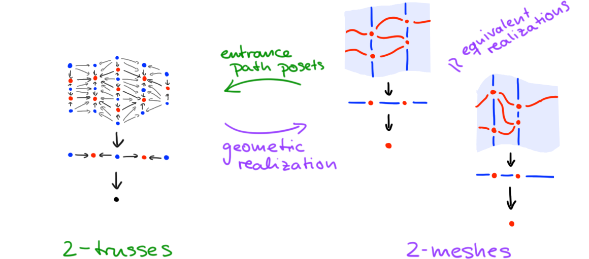
Our discussion of 1-trusses was strongly geometrically motivated by the idea of 1-meshes (as framed stratified connected \(k\)-manifolds, \(k \leq 1\)): this geometric interpretation carries over to higher dimension \(n\) as well. An \(n\)-mesh is a tower of 1-mesh bundles over the point. Maps of such \(n\)-meshes are, fully analogous to our definition in the case of \(n\)-trusses, maps of towers which fiberwise restrict to maps of 1-meshes—note that these maps have a topology making the category of \(n\)-meshes an \(\infty\)-category. Passing to entrance path posets defines a functor from the category of \(n\)-meshes to the category of \(n\)-trusses. This functor is an equivalence: its inverse is geometric realization. Technically, to spell out this equivalence in full generality, we would have to take into account \((\infty,2)\)-categorical structure (the category of posets is a 2-category). However, in the special case of closed trusses and singular maps (and, dually, open trusses and regular maps) 2-categorical structure trivializes, and we arrive at the following result.
Theorem ([1], Section 4.2). The \(\infty\)-category of closed \(n\)-meshes and the 1-category of \(n\)-trusses, both with singular maps, are equivalent. Dually, this holds in the open-regular case. \(\blacklozenge\)
We illustrate the equivalence of categories in Figure 7, in the case of an open 2-truss: the 2-truss geometrically realizes to (a contractible \(\infty\)-groupoid of) open 2-meshes; conversely, passing to the entrance path posets of these 2-meshes (and recording strata dimension and framing accordingly) recovers the 2-truss that we started with.
Computads and diagrams
In what is effectively “part II” of this note, we now turn our attention away from “local” structures and towards “global” structures. Namely, we will discuss computads which are presheafs on trusses—or, more precisely, on the “atomic cells” that constitute trusses. We will refer to these cells as “blocks”.
Block sets
Blocks are the “atomic building blocks” of closed trusses: the reader may think of them as trusses with a single facet (that is, a single cell that is not in the boundary of another cell).
Definition (Blocks). An \(n\)-truss \(k\)-block \(B\) is a closed \(n\)-truss such that
- the top poset \(B_n\) as a minimal element, called the facet of \(B\),
- \((n-k)\) of the 1-truss bundles \(p_i : B_i \to B_{i-1}\) are the identity.
The dimension vector of \(B\) is the Boolean \(n\)-vector \((d^B_1,d^B_2,...,d^B_n)\) where \(d^B_i = 0\) if \(p_i = \id\) and \(d^B_0 = 1\) otherwise. A block is called vertical if its dimension vector is of the form \((0,...,0,1,...,1)\). \(\blacklozenge\)
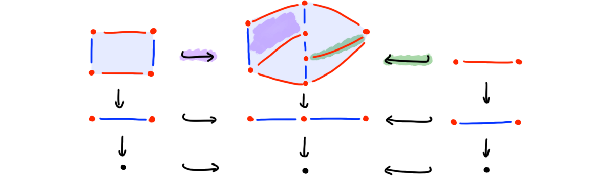
Construction (Blocks in trusses). Given an \(n\)-truss \(T\) and an element \(x \in T_n\), then restricting the tower of bundles defining \(T\) to the upper closure \(T^{\geq x}_n \into T_n\) of \(x\) defines an \(n\)-truss \(k\)-block \(T^{\geq x} \into T\). We call \(T^{\geq x}\) the face block of \(x\). \(\blacklozenge\)
Example (Blocks in trusses). In Figure 8 we depict (the geometric realizations of) a 2-truss 2-block resp. a 2-truss 1-block, both of which include as face blocks into their “parent” \(2\)-truss (shown in the middle).
Definition (Block category and block nerve). Write \(\blcat n\) for the category of \(n\)-truss blocks and singular maps (which is a subcategory of \(\sctruss n\), defined earlier). \(\blacklozenge\)
Note that (like \(\sctruss n\)) maps in \(\blcat n\) are generated by face and degeneracy maps. we will use this category in a very similar vein as other categories of “shapes” such as, for instance, the category \(\Delta\) of simplices.
Definition (Block sets). A presheaf on the category of \(n\)-truss blocks \(\blcat n\) is called a block \(n\)-set (or simply, a “block set”). The category of such presheafs will be denoted by \(\blset n = \mathrm{PSh}(\blcat n)\). \(\blacklozenge\)
Note that, while morally similar, blocks behave differently from other categories of shapes in many ways. For instance, they do not form a Reedy category in the obvious way (when ordering blocks by dimension). They also fail to be an Eilenberg-Zilber category.
Observation (Non-EZ block sets). Given a block in a block set \(X\), i.e. a map \(b : B \to X\) out of a representable, we say \(b\) is degenerate if it factors by a degeneracy \(B \to B'\) through another block \(b' : B' \to X\). It need not be the case that \(b\) is a degeneracy of a unique non-degenerate block. \(\blacklozenge\)
In light of the previous observation, it makes sense to require the following sheafiness condition, which guarantuees that block sets preserve “stratified gluings” of blocks; concretely, “stratified gluings” refers to colimits that are computed on entrance path posets in the following sense.
Definition (Geometric block sets). A geometrically absolute colimit in \(\blcat n\) is a colimit that is preserved under the functor \(\blcat n \to \Pos_n\) (here, \(\Pos_n = \Fun([n],\Pos)\) denotes \(n\)-simplices in \(\Pos\), and the functor \(\blcat n \to \Pos_n\) takes 1-truss bundles to underlying poset maps). A block set called geometric if it maps geometrically absolute colimits in \(\blcat n\) to limits in \(\SetCat\). \(\blacklozenge\)
Blocks in geometric block sets are degeneracies of unique non-degenerate blocks.
Computads
We can now define computads. Note that we use the term “(geometric) computad” not in the traditional (already-defined!) sense, but to mean a notion of “free (associative) weak higher category”.
Definition (Computads). An \(n\)-computad is an \(n\)-truss geometric block set whose non-degenerate blocks are vertical. \(\blacklozenge\)
Dropping the condition of verticality, the definition generalizes to a notion of “\(n\)-fold computad” (note also that the term “vertical” alludes to \(n\)-fold category lingo; relatedly, see also cat-\(n\)-groups and crossed \(n\)-cubes)). We will come back to \(n\)-foldness in a moment, after having discussed morphisms in computads.
A non-degenerate \(n\)-truss \(k\)-block in an \(n\)-computad can be, in traditional category theory terminology, be understood as a generating \(k\)-morphisms. The process of adding generating \(k\)-morphisms can be understood inductively: generating \((k+1)\)-morphisms are the “relations” satisfied by composites of \(k\)-morphisms (in particular, to describe a traditional \(n\)-category you would want to consider \((n+1)\)-computad, in order to capture the compositional relations satisfied by \(n\)-morphisms). Every \(n\)-computad is trivially an \((n+1)\)-computad by “categorical extension” as follows.
Construction (Embeddings). There’s an inclusion of categories \(\iota : \truss n \into \truss {n+1}\) which takes an \(n\)-truss \(T\) and augments it by a trivial bundle \(p_{0} : T_0 = T_0\) to obtain an \((n+1)\)-truss. This restricts to an inclusion \(\iota : \blcat n \into \blcat {n+1}\). \(\blacklozenge\)
Definition (Categorical truncation and extensions). Precomposition with \(\iota\) defines a functor \(\iota^\ast: \blset {n+1} \to \blset n\) called categorical truncation. Its left adjoint \(\iota_\ast : \blset n \to \blset {n+1}\) is called categorical extension. \(\blacklozenge\)
Let us now define what “morphism” in a computad are (the definition equally applies, more generally, to \(n\)-fold computads). The idea is, of course, that “shapes” are given by blocks and “diagrams of shapes” are given by trusses: therefore, we first note that trusses themselves are block sets (in fact, geometric block sets).
Construction (Block nerves). The restricted Yoneda embedding of the inclusion \(\iota : \blcat n \into \sctruss n\) induces a functor \(N = \sctruss n (\iota-,-) : \sctruss n \to \blcat n\) which we call the block nerve. \(\blacklozenge\)
Remark (Blocks build trusses). Given a truss \(T\) we have
\[T = \mathrm{colim}(\blcat n / T \to \sctruss n)\]where \(\blcat n / T \to \sctruss n\) is the forgetful functor form the comma category \(\blcat n / T\). The reader familiar with the general notion of nerves will know that there are equivalent ways to state this remark: namely, it is equivalent to the observation that the functor \(\blcat n \into \sctruss n\) is dense; it is also equivalent to the observation that the block nerve functor \(N\) is fully faithful. \(\blacklozenge\)
We say a truss \(T\) is \(k\)-vertical if \(k\) is the smallest index such that \(T\) lies in the image of \(\truss k \into \truss n\) (equivalently, its bundles \(p_i\) satisfy \(p_i = \id\) exactly for \(i \leq n-k\)).
Definition (Morphisms in computads). The \(k\)-morphisms in an \(n\)-computad \(X\) are maps \(NT \to X\) for a \(k\)-vertical \(n\)-truss \(T\). \(\blacklozenge\)
Remark (\(n\)-fold computads). Dropping the notion of \(k\)-verticality makes sense if the target \(X\) is an \(n\)-fold computad (and thus itself may contains non-vertical generating blocks): in this case, we get \(2^n\) “types of morphisms” indexed by Boolean \(n\)-vectors that record the positions of trivial bundles \(p_i = \id\) in the truss \(T\).
Problem (Computads). An open problem is the comparison of the category of computads (of which, here, we only defined its objects) to other models of higher categories (from our discussion in an earlier note about the different higher categorical paradigms in use, one may expect this to be not as “straight-forward” as other comparison results). Note that we forego a more in-depth discussion of functors of computads, but that further discussion of functors can be found in this note. \(\blacklozenge\)
Addendum (Definitional disclaimer). The definition of computads given here is tentative, and certainly other definitions are possible (e.g., together with Lukas Heidemann, we are thinking about representing computads as cofibrant objects in a model structure on block/truss sets). \(\blacklozenge\)
Pasting Diagrams and combinatorial manifold diagrams
Finally, let us formally answer two questions that have been posed in previous notes but so far only addressed “informally” (or “geometrically”); namely:
- What is a computadic pasting \(n\)-diagram?
- What is a (combinatorial) manifold \(n\)-diagram?
The answer to these questions has a further refinement: we will distinguish diagrams that are “unscoped” and “scoped” (in a computad \(X\)). Let us first observe the following. Just as cell complexes have face posets (describing the incidence relation of their faces), computads have posets describing incidence relations of blocks: of course this is a variation of the idea of entrance path posets.
Construction (Entrance and exit path posets of computads). Given a computad \(X\), its entrance path poset \(\Entr(X)\) is the poset of non-degenerate blocks in \(X\) with and arrow \(b \to c\) whenever some degeneracy of \(c\) is a face of \(b\). Its dual, is the exit path poset \(\Exit(X) = \Entr(X)\op\) of \(X\).
Given a \(k\)-morphisms \(f : NT \to X\), we obtain the \(\Exit(X)\)-labeling \(\Exit(f) : T \to \Exit(X)\) which maps \(x \in T\) to the unique nondegenerate block to which the block \(NT^{\geq x} \into NT \xto f X\) degenerates. The opposite of \(\Exit(f)\) will be denoted by \(\Entr(f) : T \to \Entr(X)\). \(\blacklozenge\)
Definition (Scoped pasting diagrams). Given an \(n\)-computad \(X\), an \(X\)-scoped pasting diagram is a \(\Exit(X)\)-labeled \(n\)-truss \(T\) where \(\lbl_T\) is of the form \(\Exit(f)\) for some (necessarily unique) higher morphism \(f : NT \to X\) in \(X\). \(\blacklozenge\)
Definition (Pasting diagrams). An unscoped pasting \(n\)-diagram is a stratified truss \(T\) for which there exists some (non-unique) morphism \(f\) in some \(n\)-computad \(Y\) such that \(\lbl_T\) is the connected component splitting of \(\Exit(f)\). \(\blacklozenge\)
We often refer to “unscoped pasting diagrams” simply as “pasting diagrams”. Note that, given an unscoped pasting \(n\)-diagram \(T\), there is always a canonical choice of \(f\) and \(Y\); namely, the “free \(n\)-computad” generated by \(Y\). This is characterized by the property that \(\Exit(f) : T \to \Exit(Y)\) is a bijection, in which case we usually write \(\Exit(Y) \equiv \Exit(T)\).
Construction (Source and targets). Let’s construct some familiar ideas: namely, “sources” and “targets” of pasting diagrams (we discuss the unscoped case, the scoped case works similarly). Let \(T = (\und T, \lbl_T)\) be a pasting diagram. Let \(\partial_\pm T_1 \into T_1\) be the endpoints of the 1-truss \(T_1\) (with frame order \((T_1,\fleq)\)). Restricting the tower of \((n-1)\) bundles \((p_n : T_n \to T_{n-1},...,p_2 :T_2 \to T_1)\) over these objects \(\partial_\pm T_1\), augmenting the resulting towers with another trivial bundle, and restricting the labeling \(\Exit(f)\) accordingly, we obtain the \(n\)-trusses \(\partial_\pm T \into T\); these are called the source and target of \(T\). \(\blacklozenge\)
Remark (Degeneracy-free diagrams). A labeled closed \(n\)-truss \(T\) is called normalized if for any degeneracy \(F : T \to S\) (which preserves labels, i.e. \(\lbl_F = \id\)) we have \(F = \id\). (Dually, this applies to open trusses and their label-preserving coarsenings). Every labeled closed \(n\)-truss admits a unique degeneracy \(T \to S\) such that \(S\) is normalized (this shown e.g. in [2]). As a consequence, each pasting diagram degenerates to a unique pasting diagram in which degenerate blocks (or, categorically, “identities”) have been maximally removed. \(\blacklozenge\)
Before finally, giving some example, let us now dualize the notion of pasting diagrams to obtain a notion of combinatorial manifold diagrams.
Definition (Scoped combinatorial manifold diagrams). Given a computad \(X\), an \(X\)-scoped combinatorial manifold diagram \(M\) is a stratified open \(n\)-truss whose dual \(M^\dagger = (\und M^\dagger, \lbl_m\op)\) is an \(X\)-scoped pasting diagram. \(\blacklozenge\)
Definition (Combinatorial manifold diagrams). An (unscoped) combinatorial manifold diagram \(M\) is a stratified open \(n\)-truss whose dual \(M^\dagger\) is a (unscoped) pasting diagram. \(\blacklozenge\)
What is the connection of such “combinatorial manifold diagrams” with the “geometric” manifold diagrams defined in an earlier note? This is where the geometric realization of \(n\)-trusses as \(n\)-meshes comes into play.
Construction (Geometric realization). Given a combinatorial manifold diagram \(M = (\und M,\lbl_M : \und M_n \to \Entr(M))\), its geometric realization \(\abs{M}\) is the stratification with characteristic map:
\[\abs{\und M} \to \und M \xto {\lbl_M} \Entr(M)\]where the first map is the characteristic map of the open \(n\)-mesh \(\abs{\und M}\) realizing the open \(n\)-truss \(\und M\) (in particular, the underlying space of \(\abs{M}\) is the same as that of \(\abs{\und M}\): the open \(n\)-cube). Note that in the \(X\)-scoped case, we would replace \(\lbl_M\) in the above with the connected component splitting of the labeling \(\lbl_M : \und M \to \Entr(X)\).
Geometric realization produces a correspondence between the following combinatorial and geometric notions:
\[\footnotesize \left\{ \begin{matrix} \text{combinatorial} \\ \text{manifold diagrams} \\ \text{that are normalized} \end{matrix} \right\} \iso \left\{ \begin{matrix} \text{geometric manifold} \\ \text{diagrams up to framed} \\ \text{stratified homeomorphism} \end{matrix} \right\} .\](The result, in the more general case of framed stratifications, is discussed in [1], Chapter 5).
Note that the construction verbatim applies to define geometric realizations of pasting diagrams as well (in this case, underlying spaces are those of closed \(n\)-meshes). \(\blacklozenge\)
Finally, examples!
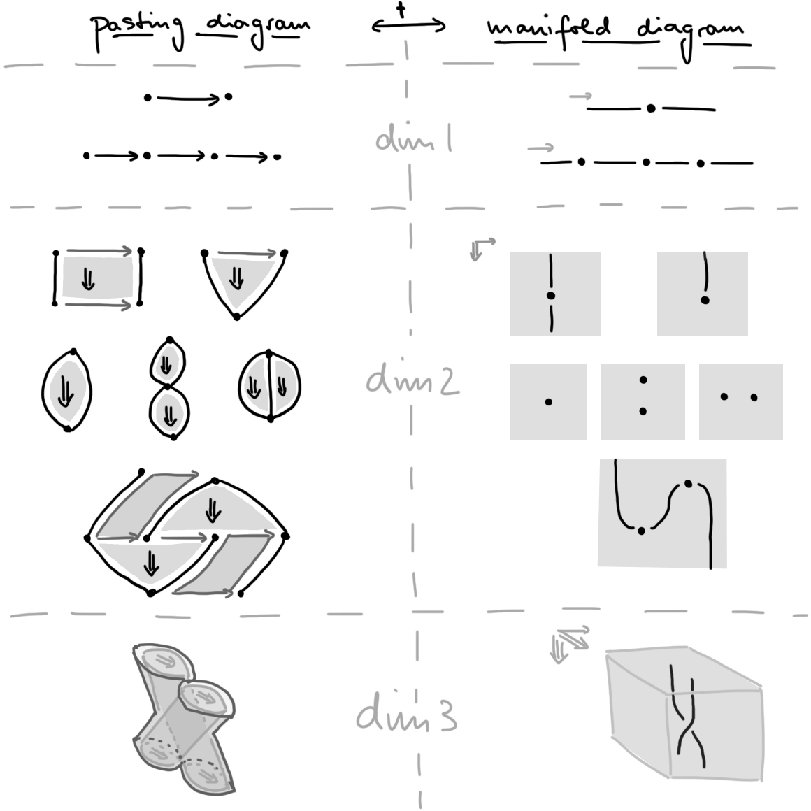
Examples (Pasting diagrams and their dual manifold diagrams). In Figure 9 we illustrate (geometric realizations of) pastings diagrams and their dual manifold diagrams. In each case we illustrate the geometric realization \(\abs{T}\) of a given labeled \(n\)-truss (whether pasting or manifold diagram): to distingsuish strata in these stratifications we either leave ample space between them or use different shades. A recipe to combinatorially interpret the pictures is as follows: (1) find the coarsest open mesh \(\abs{\und M}\) refining one of the given manifold diagrams \(\abs{M}\) (note we use arrows here and there to indicate framing directions), (2) passing to entrance path posets, build an open truss \(\und M\), (3) derive a labeling \(\lbl_M = \Entr(\abs{\und M} \to \abs{M})\) from the action of the coarsening \(\abs{\und M} \to \abs{M}\) on entrance path posets; as a result, obtain a combinatorial manifold diagram \(M = (\und M,\lbl_M)\), (4) dualize to obtain a pasting diagram \(M^\dagger\) (of course, one may also start with building closed meshes for the given geometric pasting diagrams). We leave details to the reader as a fruitful exercise. \(\blacklozenge\)
That’s it for now—as always, comments are most welcome!
References
[1] “Framed Combinatorial Topology”, Dorn + Douglas
[2] “Associative \(n\)-categories”, Dorn