
The categorical Pontryagin-Thom construction
Abstract. The Pontryagin-Thom construction is a deep relation between smooth manifold theory and homotopy theory. We use the language of manifold diagrams and computads to give a purely combinatorial perspective on the construction. On our way, we’ll discuss computadic functors and transformations, and how the combinatorics of manifold diagrams may provide a “combinatorialization” of smooth structures on manifolds altogether.
This note is part of a series.
Introduction
The classical Pontryagin-Thom construction ties together the smooth cobordism groups of framed (or otherwise structured) manifolds with the homotopy groups of spheres (or other, corresponding spectra). For an introduction to the construction, of which there are many good ones, see for instance ([1], Chapter 1) or ([2], Chapter 8). To see why this bridge between two fields is so interesting, consider the following two points.
-
The PT construction conceptually underlies our algebraic understanding of (framed) manifolds and their cobordisms, leading for instance to (framed) surgery theory, see [1] (it is therefore related to prominent surgery-theoretic problems such as the Kervaire invariant one problem). In particular, it currently provides a main approach in understanding exotic smooth structures relating, for example, exotic smooth structures of spheres to stable homotopy groups (see loc. cit.).
-
Conversely, via the PT construction, the geometry of smooth manifolds affects our understanding of homotopy-theoretic structures. It leads, for instance, to the construction of Thom spaces and spectra. It also provides a differential-topological understanding of classical theorems such as the Freudenthal suspension theorem, see [1]. More generally, if we take “homotopy theory” to mean \((\infty,n)\)-category theory, the PT construction conceptually underlies guiding paradigms such as the the tangle, the cobordism and the stabilization hypotheses.
-
Mike Hopkins names Pontryagin’s insight into the relation of framed cobordism and homotopy groups as the birth of modern Algebraic Topology (see minute 1:08 of the interview), … that should mean something!
While ubiquitous in many places (and in many forms), the PT construction is rarely fledged out in full foundational detail—instead, one requires a “fair amount of technical skill to fill in the details” regarding the needed differential topological tools (see [2]). The purpose of this note is to sketch a purely combinatorial (in fact, categorical) approach to the PT construction, expressed in a different foundational framework than that of differential point-set topology; namely, we will use the language of manifold diagrams based on framed combinatorial topology. As we will discuss, capturing smooth manifold in terms of manifold diagrams in this way should lead to a combinatorialization of smooth structures (this perspective is somewhat implicit in the combinatorial approach to singularity theory and “higher” Morse theory discussed in a previous note).
More on computads
The categorical PT construction will turn functors between computads into stratifications of computads. Our first goal will therefore be the definition of functors of computads.
Recall from our discussion of trusses that (closed) \(n\)-trusses are “built out of” \(n\)-truss \(k\)-blocks. Recall, block \(n\)-sets are (\(\SetCat\)-valued) presheafs of \(n\)-truss blocks. From this we obtained a notion of (weak) \(n\)-computads by requiring geometric colimits to be preserved and generating blocks to be vertical. Here, we will sometimes refer to the \(n\)-truss \(k\)-blocks of an \(n\)-computad also as (computadic) \(k\)-cells (to invoke the classical picture of cell complexes in the reader’s mind).
Functors
A functor of computads \(C \to D\) will map “generating morphisms” in \(C\) to “morphisms” in \(D\). Here, the non-degenerate cells of a computad are considered to be its generating morphisms. The process of generating other morphisms from generating morphisms also has a precise description: recall, a \(k\)-morphism in an \(n\)-computad \(D\) is a a map of block sets \(NT \to D\) from the block nerve \(NT\) of a \(k\)-vertical closed \(n\)-truss \(T\) (equivalently, this is a \(D\)-scoped pasting diagram).
Recall also that closed trusses (and thus truss blocks) come not only with notions of faces and degeneracies but also their dual counterparts: namely, embeddings and subdivisions. A subdivision of \(T \to B\) of a block \(B\) by a truss \(T\) can be thought of as cutting the block \(B\) into smaller blocks (which assemble into the truss \(T\)). A functor of computads \(C \to D\) will map cells of \(C\) to morphisms of \(D\) by first subdividing cells in \(C\), and then labeling the subdivisions with cells in \(D\). We give the definition in the following slightly more general form (which applies to block sets in general).
Definition (Functors). Given block \(n\)-sets \(C\) and \(D\), a functor \(F : C \to D\) associates to each non-degenerate cell \(b : B \to C\) in \(C\) a subdivision \(\subdiv_b : T \to B\) of \(B\) by an \(n\)-truss \(T\), and a block set map \(\lbl_b : NT \to D\) which ‘labels’ \(T\) in \(D\). This must be compatible with faces: for any face \(a : A \to C\) of \(b\) (that is, \(a = b \circ f\) with \(f : A \hookrightarrow B\)) we have \(\subdiv_a = f^{\ast}\subdiv_b\) and \(\lbl_a = \lbl_b \circ \subdiv^{\ast}_b f\). Our notation refers to the following pullback square:
\[\begin{CD} S @>{\subdiv^{\ast}_b f}>> T \\ @V{f^{\ast}\subdiv_b}VV @VV{\subdiv_b}V \\ A @>f>> B. \end{CD}\]If both \(C\) and \(D\) are computads, we speak of a functor of computads. \(\blacklozenge\)
(There are variations of this definition, depending on how exactly one wants to use subdivisions. The above phrasing is convenient to us here.)
Remark 1 (Composition of computad functors). We will forego a discussion of composition of functors of computads. The reader trying to write down such a definition might find the following: instead of a strict notion of composition, which produces a composite \(H = F \circ G\), functors of computads naturally compose weakly, yielding an equivalence class of composition candidates \(H\) (namely, up to “natural homotopy”, which we define below). \(\blacklozenge\)
Cylindrical transformations
A cylindrical transformations is a functor of the form \(C \times I \to D\) where \(C \times I\) is the “cylinder” of an \(n\)-computad \(C\), and \(D\) is an \((n+1)\)-computad.
Definition (Cylinders of blocks). Given an \(n\)-truss block \(B\), the cylinder block \(B \times I\) is the \((n+1)\)-truss block consisting of a tower of 1-truss bundles
\[(B \times I)_{n+1} \to (B \times I)_n \to ... \to (B \times I)_1 \to \ast\]such that \((B \times I)_1\) is the unique 1-truss 1-block \(I\) (the “interval”), and such that the remaining \(n\)-truss bundle over \((B \times I)_1\) is the constant \(B\)-bundle, that is, it is classified by the constant map \((B \times I)_1 \to \ttr n\) mapping to \(B \in \ttr n\). We obtain a functor
\[(- \times I) : \blcat n \into \blcat {n+1}\]from \(n\)-blocks to \((n+1)\)-blocks by applying maps of \(n\)-blocks fiberwise over \((- \times I)_1 = I\). \(\blacklozenge\)
Recall also that there is also an inclusion \(\iota : \blcat n \into \blcat {n+1}\), given by augmenting an \(n\)-block \(B\) with the trivial truss bundles \(B_0 \to B_0\) at its end. Note that the source and the target of \(B \times I\) both equal the \((n+1)\)-block \(\iota B\); we denote the corresponding face maps of \((n+1)\)-blocks by \(\partial^+ : \iota B \into B \times I\) respectively \(\partial^- : \iota B \into B\). We obtain two natural transformations
\[\partial^\pm : \iota \imp (- \times I).\]Taking the cylinder of a block set does the expected: it builds a block set by taking cylinders of all blocks of a given block set, while preserving face and degeneracy structure appropriately. This may be formalized as follows. First, note that given an block \((n+1)\)-set \(C\) we may precompose \(C\) with either of the above functors \(\iota\) and \((- \times I)\) to obtain an \(n\)-computad. Recall, \(\iota^* C\) is called the \(n\)-truncation of \(C\). We will call \((- \times I)^* C\) the \(n\)-computad of cylindrical cells in \(C\).
Definition (Cylinders of block sets). Given a block \(n\)-set \(C\), its cylinder \(C \times I\) is the smallest block \((n+1)\)-set such that
- the \(n\)-truncation \(\iota^* (C \times I)\) is the coproduct of two copies of \(C\) (witnessed by inclusions \(\rho^\pm : C \into \iota^* (C \times I)\))
- \(C \times I\) itself contains “cylinder” cells for all cells of \(C\) (i.e. an iso \(\sigma : C \iso (- \times I)^* (C \times I)\))
- subject to the condition that \((C \times I)(\partial^\pm) \circ \sigma = \rho^\pm\) commutes. \(\blacklozenge\)
Remark 2 (Cylinders aren’t globular). Cylinders of computads are generally not computads themselves: indeed, it should be intuitively clear that already taking the product of a single computadic \(k\)-cell \(C\) with an interval \(I\) doesn’t result in another computadic \((k+1)\)-cell (as the product creates non-vertical boundaries for the resulting non-degenerate \((k+1)\)-block). \(\blacklozenge\)
The definition of cylindrical transformations now takes the following form.
Definition (Cylindrical transformations). Consider functors \(F, G : C \to \iota^* D\) from an \(n\)-computad \(C\) to the \(n\)-truncation \(\iota^* D\) of an \((n+1)\)-computad \(D\). A cylindrical transformation \(\alpha : F \imp G\) is a functor of \((n+1)\)-computads \(\alpha : C \times I \to D\). \(\blacklozenge\)
Remark 3 (Cylindrical vs natural transformations). Cylindrical transformation are natural transformations in which all components of the natural transformations below dimension \(n+1\) are homotopies (that is, they are \(k\)-morphisms but do not contain any generating \(k\)-morphisms; the idea was sketched in an earlier note). This may be confusing, since natural transformations are also defined as functors \(C \times I \to D\): however, the product ‘\(\times\)’ in the latter definition is not the same as the cylinder construction above. (Instead, an attempt to translate the cylinder construction into classical lingo would have to refer to products of \(n\)-fold categories).
Of course, it also makes sense to speak of cylindrical equivalences \(\alpha : F \iso G : C \to D\) if all components of a cylindrical transformation \(\alpha\) are equivalences. (Note that for a notion of “equivalence” one would usually require \(D\) to be the truncation of an even higher computad, at least of dimension \(n+2\), which then allows us to determine whether a given \((n+1)\)-morphisms is an equivalences.) If an \(n\)-computad \(D\) is given trivial higher structure (formally by applying the left adjoint \(\iota_{\ast}\) of \(\iota^{\ast}\) enough times) then this specializes to a notion of natural homotopy (since the only invertible higher morphisms are homotopies in this case).
The categorical PT construction
Given a functor of \(n\)-computads \(F : C \to D\) we construct a stratification of \(C\) (defined in combinatorial terms). By the same mechanism, given a cylindrical transformation \(F : C \times I \to D\) we will stratify the cylinder \(C \times I\). The construction takes the following simple form.
Construction (Categorical PT construction). Given a functor of \(n\)-computads \(F : C \to D\), by definition, each non-degenerate cell \(b : B \to C\) is subdived by a truss \(\subdiv_b : T \to B\). That truss (after taking its block nerve) maps into \(D\) by a block set map \(\lbl_b : NT \to D\). As we’ve seen, this induces a map of posets \(\Exit(\lbl_b) : T_n \to \Exit(D)\), where \(\Exit(D)\) is the exit path poset of \(D\) (consisting of non-degenerate blocks and incidence relations): namely, each element \(x \in T_n\) determines a face block \(T^{\geq x} \into T\), which by the block set map \(\subdiv_b\) is mapped to some block \(a : A \to D\), which in turn is a degeneracy of a unique non-degenerate block \(\Exit(\lbl_b)(a) \in \Exit(D)\). Thus, \((T, \lbl_b : T_n \to \Exit(D))\) is a labeled \(n\)-truss. As a result, we obtain a (\(D\)-scoped) pasting \(n\)-diagram \((T, \Entr(\lbl_b))\). Its dual \((T^\dagger, \Entr(\lbl_b))\) (where \(\Entr(\lbl_b) = \Entr(\lbl_b)\op\)) is a \(D\)-scoped combinatorial manifold \(n\)-diagram. This combinatorial manifold diagram provides the (combinatorial) datum of a stratification of the an open cube, which we think of as stratifying the “open interior” of the non-degenerate cell \(b : B \to C\). (By definition of computad functors, this stratification is suitably compatible with the corresponding stratifications \((S^\dagger, \lbl_c\op)\) of faces \(c\) of \(b\); details are left as an exercise!) \(\blacklozenge\)
Almost exactly the same construction can be used for cylindrical transformations \(C \times I \to D\), yielding a stratifications of the cylinder \(C \times I\)—the resulting stratifications on cells of \(C \times I\) will be called (\(D\)-scoped) manifold diagram cobordisms (note that, in particular, they are (\(D\)-scoped) manifold diagrams themselves).
Remark 4 (Geometric realization). The “combinatorial” datum of a stratification associated to a functor \(F : C \to D\) defined in the preceding construction can of course be turned into an actual stratification: recall, combinatorial manifold diagrams correspond to geometric manifold diagrams (i.e. actual stratifications of the open cube) up to framed stratified homeomorphism, and the correspondence is by a process of geometric realization. Realizing computads \(C\) as (framed) cell complexes \(\abs{C}\) of their non-degenerate cells, this can be used to geometrically stratify the open interior of cells \(\abs{b \into C}\); moreover, inducting up the skeleta of \(\abs{C}\), one can arrange these cell-wise stratifications (by appropriate framed stratified isomorphisms on each cell) to fit into a global stratification of \(\abs{C}\). \(\blacklozenge\)
Turning the above PT construction into a “PT correspondence” becomes essentially a tautology with the following definitions (which simply recast our earlier definitions of functors and cylindrical transformations of computads).
Definition (Combinatorial stratifications and cobordisms). Given an \(n\)-computad \(C\) and an \((n+1)\)-computad \(D\), a \(D\)-stratification of \(C\) is choice of \(D\)-scoped manifold diagram (dual to some \(k\)-morphism in \(D\)) for each \(k\)-cell in \(C\), suitably compatible with faces in \(C\). Similarly, a \(D\)-cobordism of \(D\)-stratifications of \(C\) is a choice of \(D\)-scoped manifold diagram for each \(k\)-cell \(C \times I\), which again is suitably compatible with faces. \(\blacklozenge\)
This leads to the following (tautological) correspondence.
The set of \(D\)-stratifications of \(C\) up to \(D\)-cobordism correspond to the set of computad functors \(C \to D\) up to cylindrical transformation. We will denote either set by \([C,D]\).
One may also wish to replace “cylindrical transformation” with “cylindrical equivalence” or “natural homotopy”, changing the definition of cobordisms accordingly (note that if \(D\) does not have any non-trivial cells in dimension \((n+1)\) then we automatically work with natural homotopies). Further to the preceding remark on geometric realization, the correspondence can also be phrased in terms of geometric stratifications and cobordisms on the (framed) cell complex \(\abs{C}\); this links our combinatorial discussion with the classical PT construction, as we will illustrate in the next examples.
Examples
We discuss the set \([C,D]\) for simple instances of computads \(C\) and \(D\).
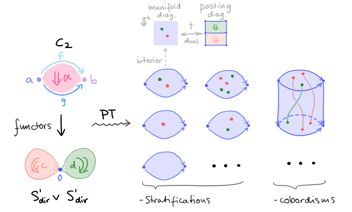
Example 1 (Wedge of directed spheres). Define the “walking 2-cell” \(C_2\) to be the \(2\)-computad with two objects \(a, b\), two 1-morphisms \(f,g : a \to b\), and a 2-morphism \(\alpha : f \imp g\). Define the “wedge of directed \(2\)-spheres” \(\vee^2 S^2_{\mathrm{dir}}\) be the computad with a single object \(0\), and two \(2\)-morphisms \(c,d : \id_0 \imp \id_0\). The set \([C_2,\vee^2 S^2_{\mathrm{dir}}]\) of \(\vee^2 S^2_{\mathrm{dir}}\)-stratifications of \(C_2\) up to cobordism is \(\lN \oplus \lN\). In Figure 1, on the left, we depict (geometric realizations) of \(C_2\) resp. \(\vee^2 S^2_{\mathrm{dir}}\). To the right, we depict stratification representatives of functors in \([C_2,\vee^2 S^2_{\mathrm{dir}}]\) as well as their cobordisms; on the top, for the first stratification, we illustrate the (\(\vee^2 S^2_{\mathrm{dir}}\)-scoped) manifold diagram stratifying the interior of \(\alpha\)—this dualizes to the shown pasting \(2\)-diagram diagram, which thus recovers the image of \(\alpha\) under the corresponding functor \(C_2 \to \vee^2 S^2_{\mathrm{dir}}\) in classical “cellular” categorical terms. (Note, since all other other generating morphisms of \(C_2\) are contained in the boundary of alpha, this manifold/pasting diagram in fact determines the functor fully.) \(\blacklozenge\)
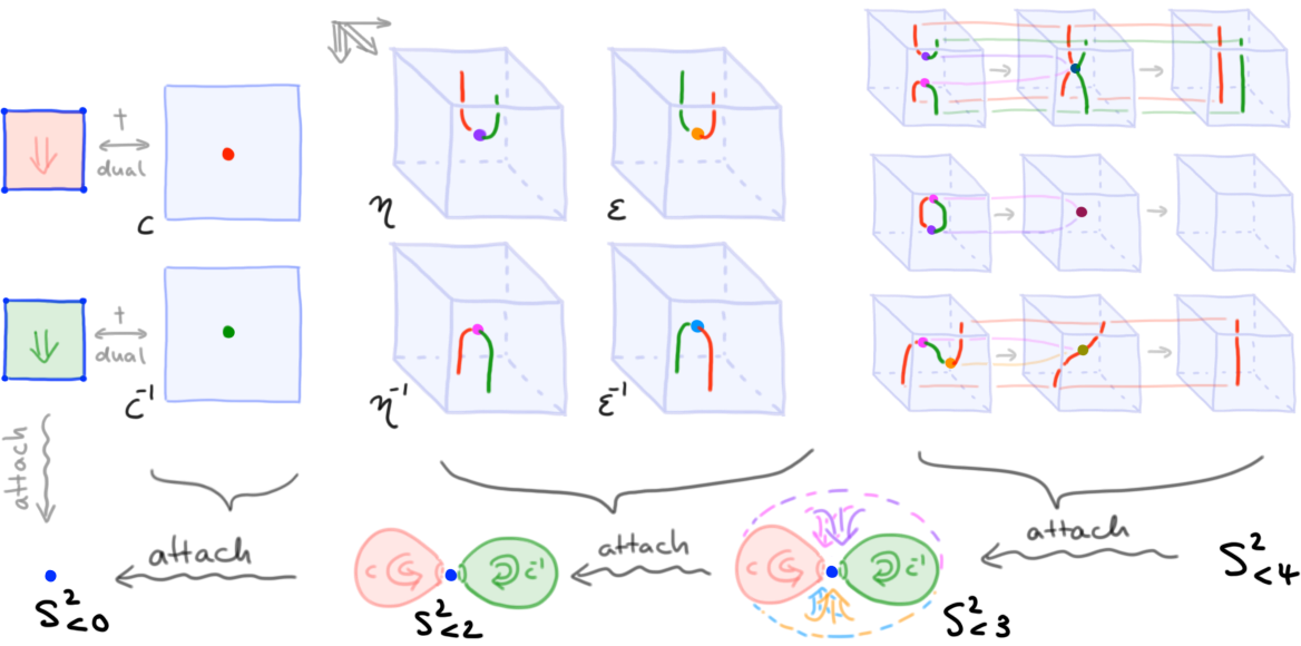
Example 2 (Cell attachments as manifold diagram singularities). Given a computad \(C\), then each non-degenerate cell \(c : B \to C\) of \(C\) canonically determines a functor of computads \(c : B \to C\) (by taking the trivial subdivision of \(B\), \(\id : B = B\)). Using the PT construction, we thus obtain a manifold diagram on the open interior of that cell; in fact, this is a manifold diagram singularity (singularities are the duals of pasting diagrams with a single cell). Moreover, this manifold diagram fully encodes the map \(c : B \to C\) (due to the assumption that \(c\) is non-degenerate). As an example, consider the following \(4\)-computad \(S^2_{<4}\), called the “homotopy \(3\)-type of the (undirected) \(2\)-sphere”. The computad consists of a single object \(0\), and a single \(2\)-cell \(c : \id_0 \to \id_0\) which is an adjoint \(2\)-equivalence. Spelling the latter condition out adds the following data: a \(2\)-morphism \(c\inv : \id_0 \to \id_0\), which is the “adjoint inverse” to \(c\), together with a “unit” \(\eta : \id^2_0 \to (c\inv \circ c)\) (which itself has inverse \(\eta\inv\)), a “counit” \(\eps : (c \circ c\inv) \to \id^2_0\) (with inverse \(\eps\inv\)) and cells for the adjunction laws of \(\eta\) and \(\eps\) as well as their inverses. These cells may be represented by manifold diagram singularities which are shown in Figure 2 (there are two \(2\)-cells, four \(3\)-cells, and sixteen \(4\)-cells; we only depict a selection of \(4\)-cells, which may be completed by applying symmetries and color-exchanges to the depicted diagrams). Note that we here and henceforth depict 4-cells in “stages”, sampling \(\lR^4\) at discrete times \(\{t\} \times \lR^3\). \(\blacklozenge\)
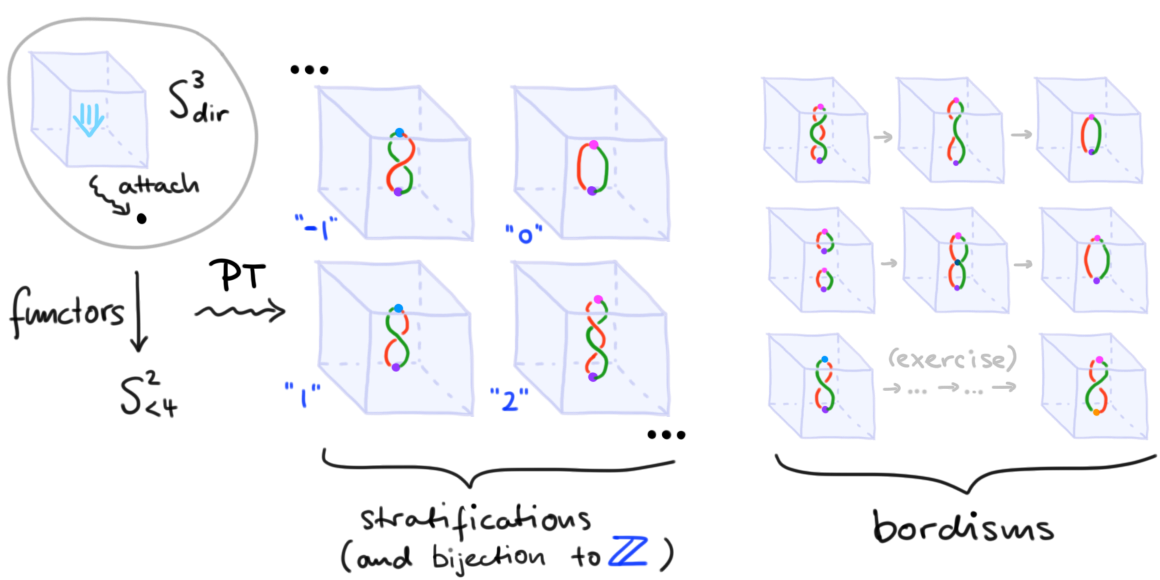
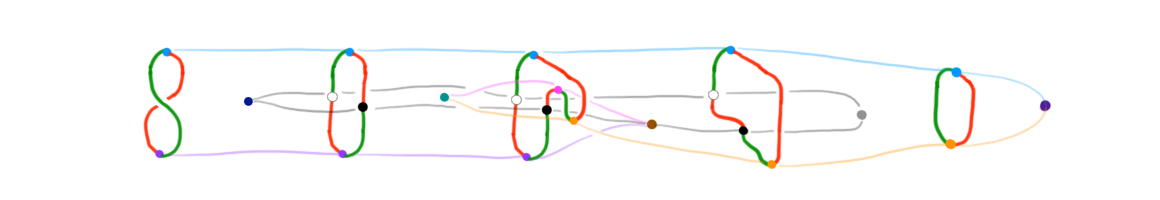
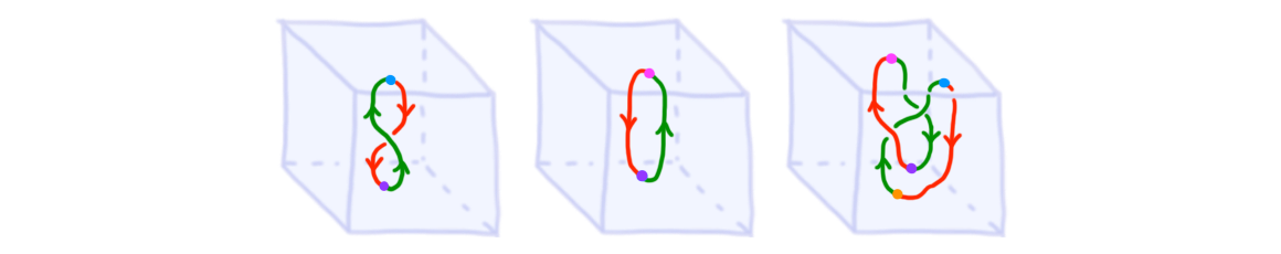
Example 3 (Computing \(\pi_3 S^2\)). Define the “the directed \(3\)-sphere” \(S^3_{\mathrm{dir}}\) to be the computad consisting of a single object, and a single \(3\)-cell. Then \([S^3_{\mathrm{dir}},S^2_{< 4}]\) (with \(S^2_{< 4}\) as in the previous example) is \(\lZ\). In fact, this combinatorial construction secretely computes the classical space of maps up to homotopy \([S^3,S^2_{< 4}] = \pi_3 S^2 = \lZ\). In Figure 3 we (geometrically) depict representatives of \([S^3_{\mathrm{dir}},S^2_{< 4}]\) (in each case, we depict functor representatives by the manifold \(3\)-diagram stratifying the \(3\)-cell of \(S^3_{\mathrm{dir}}\), and cylindrical transformations by the manifold \(3\)-diagrams cobordism stratifying the cylinder \(4\)-cell of \(S^3_{\mathrm{dir}} \times I\)). The identification \([S^3_{\mathrm{dir}},S^2_{< 4}] \iso \lZ\) takes a manifold \(3\)-diagram stratifying the 3-cell of \(S^3_{\mathrm{dir}}\) (and thus representing a functor), and maps it to the number of “\(c\inv\) over \(c\)” braids (i.e. green-over-red braids) subtracted with the number of “\(c\) over \(c\inv\)” braids (i.e. red-over-green braids) in that diagram. \(\blacklozenge\)
Normal framed cobordisms
The preceding example “almost” recovers the classical PT construction! A last piece of the puzzle is missing. Recall (e.g from [2]), the classical PT construction relates for instance
\[\Omega^{\mathrm{nfr}}_1(\lR^3) \iso \pi_3(S^2),\]that is, it relates homotopy classes of maps in \(\pi_3 S^2\) with cobordism classes of normal framed \(1\)-manifolds in \(\lR^3\). Where did the normal framing data in the preceding example go? In fact, as we now outline, this data is implicit contained in our above categorical PT construction—it roots, ultimately, in the interaction of adjoint equivalences with the intrinsic framings of cells in framed combinatorial topology.
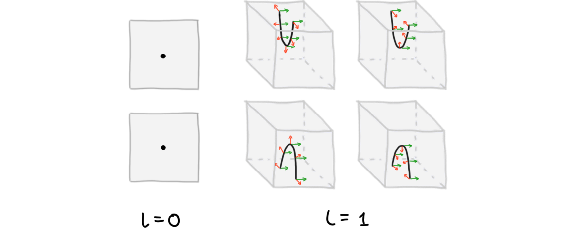
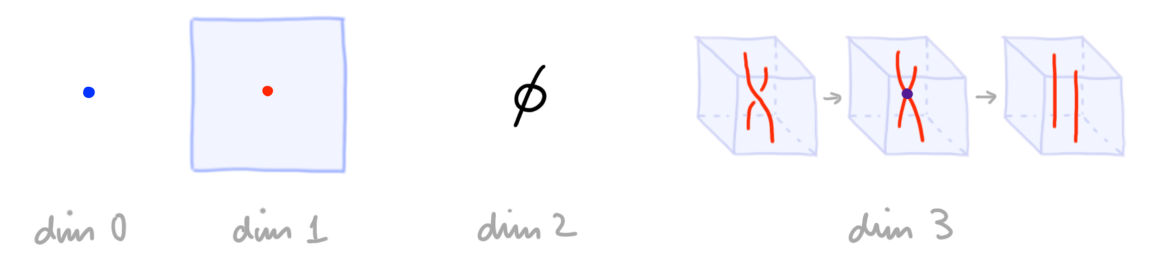
Recovering normal framing data will hinge on the following slogan: the laws that a 1-morphisms has to satisfy in order for it to be a (higher) adjoint equivalence are combinatorially described by “signed” elementary tangle singularities in codimension 1. Here, “signing” a codimension-1 tangle singularity means the following: note that each codimension-1 tangle singularity has a complement with two components; a signing simply assigns the signs ‘\(-\)’ and ‘\(+\)’ to these two components. Such an assignment can be thought of as encoding a classical normal 1-framing: namely, we can think of normal frame vectors to point from the manifold into the \(+\) component. We illustrate this in Figure 4 for signed codimension-1 elementary \(l\)-singularities, where \(l = 0,1,2\). We illustrate “classical normal frames” (derived from the signing) by vectors in red.
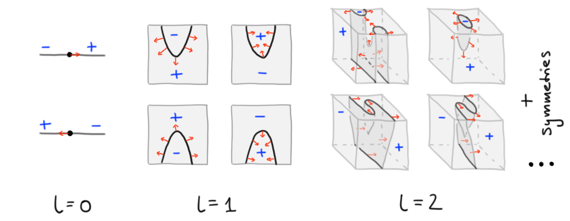
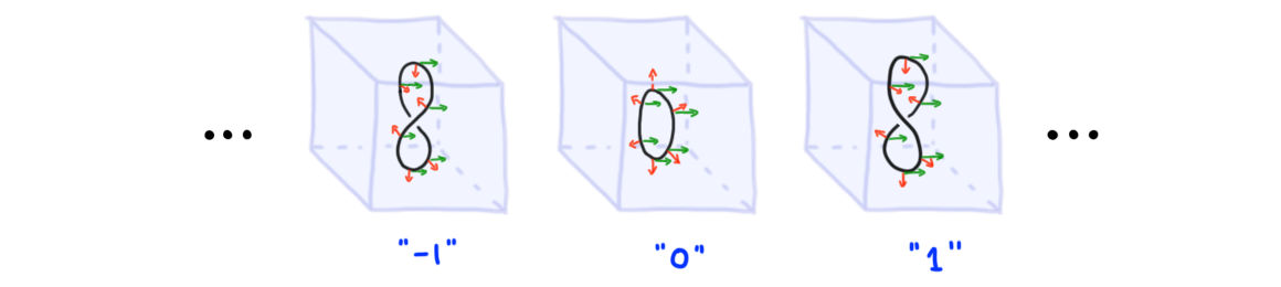
To obtain normal \(k\)-framings, for \(k \leq 1\), note that signed codimension-1 singularities can be stabilized to codimension-\(k\) singularities by an embedding \(\lR^n \iso \lR^n \times \{0\}^{k-1} \subset \lR^{n+k-1}\); normal \(1\)-framings stabilize accordingly to normal \(k\)-framings by adding \((k-1)\) trivial vector fields \(e_{n+1}, e_{n} ..., e_{n+k-1}\). We refer to the resulting singularities as signed codimension-\(k\) singularities. As an example, the six signed codimension-\(1\) elementary \(l\)-singularities on the left in Figure 4 (for \(l = \{0,1\}\)) stabilize to the six signed codimension-\(2\) elementary \(l\)-singularities in Figure 5 below.
Our previous slogan can now be turned into the following construction of cells in computads that are adjoint equivalences.
Construction (Attaching higher adjoint equivalences). Given a \(n\)-computad \(D\), let \(f_\pm : T_\pm \to D\) be \((k-1)\)-morphisms in \(D\) with equal boundary \(\partial f_- = \partial f_+\). We want to attach a new \(k\)-morphism \(c\) to \(D\) with source \(f_-\) and target \(f_+\) (write this as \(c : f_- \to f_+\)) such that \(c\) is an \((n-k)\)-equivalence. This can be achieved by attaching all signed codimension-\(k\) elementary \(l\)-singularities, \(0 \leq l \leq n-k\), as new cells to \(D\), appropriately glued to \(D\) using the boundary \(f\); in particular:
- for the signed \(0\)-singularity \(- \to +\), attach \(c : f_- \to f_+\) itself
- for the signed \(0\)-singularity \(+ \to -\), attach \(c\inv : f_+ \to f_-\)
- for the first signed \(1\)-singularity (in Fig. 4) attach a cell \(c\inv \circ c \to \id\)
- and so on for all other signed tangle \(l\)-singularities, \(l \leq n-k\). \(\blacklozenge\)
The preceding construction is a sketch (a detailed description, using older notation, can be found in [4], Section 9.1.3), but the next example hopefully further elucidates what is going on.
Example (Higher adjoint equivalence) For our earlier example of \(S^2_{<4}\) with adjoint equivalent \(2\)-cell \(c\), the six signed elementary singularities from Figure 4 are “glued in” exactly as the six cells \(c\), \(c\inv\), \(\eta\), \(\eta\inv\), \(\eps\) and \(\eps\inv\) shown in Figure 2; using stabilization of normal frames, we may think of these as having normal framings as shown in Figure 5. The remaining data of the \(2\)-cell \(c\) being an adjoint \(2\)-equivalence lies with the \(4\)-cells, and those can be understood as similarly attaching the remaining (stabilized) elementary \(3\)-singularities from Figure 4. \(\blacklozenge\)
In summary, we can (combinatorially) represent normal framings in our PT construction as follows. Assume \(D\) is a computad with a cell \(c\) that is an adjoint equivalence. By the above construction, we identify all the cells \(\{w_c\}\) witnessing that \(c\) is an adjoint equivalence with corresponding signed tangle singularities. Now, given a \(D\)-labeled manifold diagram (for example, constructed by the PT construction from a functor \(C \to D\)) we may form a manifold as the union of both strata labeled by \(c\) and strata labeled with some \(w_c\). This manifold, denote it by \(M_c\), is a tangle (since it consists of signed tangle singularities). In fact, it is a normal framed tangle: the local normal framing of each (stabilized) signed tangle singularity defines a global normal framing on all of \(M_c\).
As an example, note that the manifold \(M_c\) in each manifold diagram of Figure 3 obtains a normal \(2\)-framing: we illustrate this in Figure 6. The right picture represents the “generator” of \([S^3_{\mathrm{dir}},S^2_{< 4}] \iso \lZ\) by a normal \(2\)-framed \(1\)-manifold in \(\lR^3\): the normal framing “twists” around when traveling along the manifold once (this precisely recovers the classical normal framed codimension-2 1-manifold constructed, up to cobordism, using the classical PT construction from generator of \(\pi_3 S^2\)).
We end with the following remark. There is, of course, a more general mechanism at play, by which our earlier example of a \(4\)-computad \(S^2_{<4}\) “models” the homotopy \(3\)-type of the \(2\)-sphere \(S^2\). This can be sketched as follows.
Remark 5 (Groupoidal computads for modeling homotopy types). An \(m\)-computad which is built by attaching only cells that are adjoint \((m-i)\)-equivalences is called a groupoidal computad. Groupoidal computads allow us to model cell complexes by the following procedure. Given a cell complex \(X\), we inductively build an \(m\)-computad \(X_{\leq m}\) modeling the homotopy \((m-1)\)-type of \(X\). The case \(m = 0\) is clear (\(0\)-cells of \(X\) become objects of the \(0\)-computad \(X_{<0}\)). Assume to have constructed the groupoidal \((m-1)\)-computad \(X_{<m-1}\). By adding further adjoint equivalence data in dimension \(m\) (for previously attached cells) we may think of \(X_{<m-1}\) as a groupoidal \(m\)-computad. Now, for each \(m\)-cell \(c\) of \(X\), with attaching map \(f : S^{m-1} \to X\), we attach a new adjoint equivalent \(m\)-cell \(c : f_- \to f_+\) to \(X_{<m-1}\) such that, after geometric realization, the attachment maps \(f\) of \(c\) in \(X\) and the realized boundary \(\abs{f_- \cup_{\partial f_\pm} f_+}\) of \(c\) in \(\abs{X_{<m-1}}\) coincide up to homotopy (in the category of homotopy \((m-1)\)-types). Note that \(c\) being an adjoint equivalent \(m\)-cell in an \(m\)-computad means that so far it only has an inverse \(c\inv\); but “higher” equivalence data will be added later in the inductive process. Note also that there’s some creative freedom in this process:
- We consider attaching maps only “up to homotopy”.
- The boundary decomposition \(f \equiv f_- \cup_{\partial f_\pm} f_+\) into source and target of \(c\) can be chosen freely (this freedom cascades into lower dimension for cells in \(f_\pm\)). \(\blacklozenge\)
Disclaimer (Omitting framings). For simplicity, in the preceding remark and henceforth, we ignore normal framings of strata (which are, however, a central part of the story). A more refined account of the situation is given in section 8 of these notes.
The family of cobordism theories
In the previous section we have outlined how functors of computads \(C \to D\) (where cells of \(D\) are adjoint equivalences) produce normal framed \(D\)-stratifications on \(C\). “Framings” are the most basic of all structures on manifolds, and in a precise sense all other structures on manifolds can be obtained by “further building” on framings. We will explain how, in purely categorical terms, we can understand such structured manifolds.
Classically, we can adapt the PT construction from the case of normal framed bordism groups (yielding the isomorphism \(\Omega^{\mathrm{nfr}}_k (\lR^{n+k}) \iso \pi_{n+k}(S^n)\)) to normal \(G\)-structured bordism groups, yielding an isomorphism (see [2])
\[\Omega^{G}_k (\lR^{n+k}) \iso \pi_{n+k}(\mathbf{M}G(n)).\]Here, \(G(n) \to O(n)\) is some structure group mapping to the orthogonal group \(O(n)\) (the structure group of “bare”, i.e. “unstructured”, smooth \(n\)-vector bundles), and \(\mathbf{M}G(n)\) is the Thom space of the associated \(n\)-vector bundle \(EG(n) \times_{G(n)} \lR^n \to BG(n)\) of the \(G(n)\)-universal principal bundle \(EG(n) \to BG(n)\).
This generalization of the PT construction to \(G(n)\)-structures on normal bundles of \(k\)-manifolds can be translated into our categorical setting. We will need to understand the Thom space \(\mathbf{M}G(n)\) as an \((n+k)\)-computad. We’ll then be able to consider computad functors \(S^n_{\mathrm{dir}} \to \mathbf{M}G(n)\), and construct their induced manifold diagrams (on the interior of \(S^n_{\mathrm{dir}}\)) via our categorical PT construction.
These manifold diagrams will carry “combinatorially encoded”
\(G(n)\)-structures on normal bundles of manifolds they contain.
The recipe for understanding \(\mathbf{M}G(n)\) as a computad is easy: we first want to understand \(\mathbf{M}G(n)\) as a cell complex; and then we can model the attaching of its cells by corresponding attachments of adjoint equivalent computadic cells as outlined in Remark 5. Importantly, the cell structure of \(\mathbf{M}G(n)\) is related to the cell structure of \(BG(n)\) (as discussed here): any \(i\)-cell \(f : D_i \to BG(n)\) yields an \((i+n)\)-cell of \(\mathbf{M}G(n)\) given by the composite of maps
\[\begin{CD} D_i \times D_n @>>> D(EG(n) \times_{G(n)} \lR^n) @>>> \mathbf{M}G(n) \\ @VVV @VVpV @. \\ D_i @>f>> BG(n) @. \end{CD}\]where the right square is a pullback, and \(D(EG(n) \times_{G(n)} \lR^n)\) is the unit disk bundle over \(BG(n)\). Having constructed the cell structure of the Thom space \(\mathbf{M}G(n)\), the construction of the “Thom computad” \(\mathbf{M}G(n)_{<n+k}\) then follows the general procedure for modeling cell complexes given in Remark 5.
Let us walk through this recipe in three examples in dimension \(n = 2\): namely, for “orthogonal structure” \(G_2 = O(2)\), for “special orthogonal structure” \(G_2 = SO(2)\) and (again) for “framing structure” \(G_2 = \ast\). Note we will refer to “orthogonally structured” vector bundles simply as vector bundles (since \(O(n) \into \mathrm{Gl}(n)\) is an equivalence, and consequently all orthogonal structures on a bundle are equivalent), and to “special orthogonally structured” vector bundles as “oriented” vector bundles.
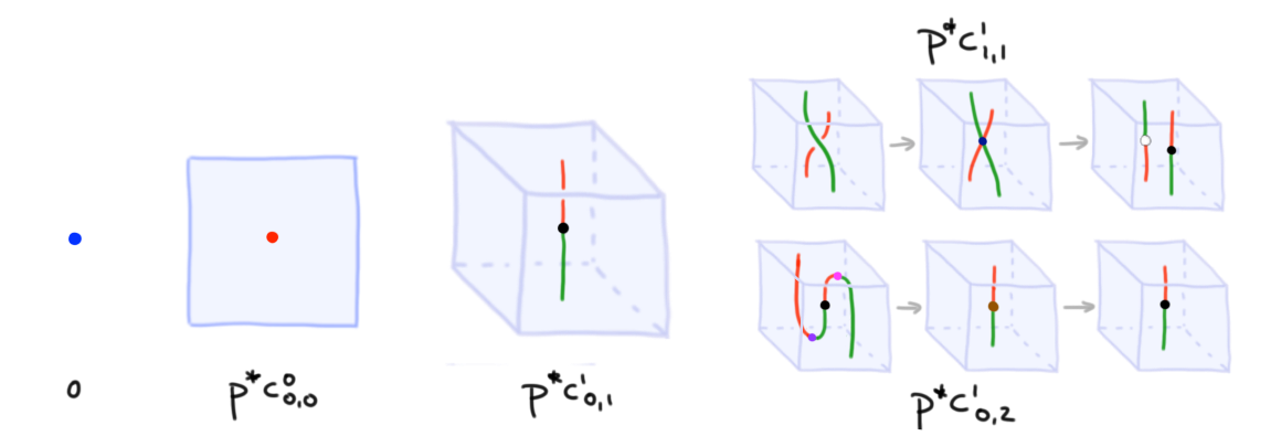
Example 4 (Smooth manifolds). We discuss the Thom computad associated to the orthogonal group \(O(2)\). By the classical PT construction, the third homotopy group \(\pi_3\mathbf{M}O(2)\) corresponds to \(\Sigma_1(\lR^3)\), that is, to smooth 1-manifolds \(M\) embedded in \(\lR^3\) up to cobordism. Following the above recipe, this can be categorically understood as follows. To build the \(4\)-computad \(\mathbf{M}O(2)_{<4}\) we need to understand the cell structure of \(\mathbf{M}O(2)\) up to dimension \(4\), and thus the cell structure of \(BO(2)\) up to dimension \(2\). The latter space is the limit of 2-plane Grassmannians \(\mathbf{Gr}(2,n)\) for \(n \to \infty\). \(k\)-Plane Grassmannians can be build from Schubert cells indexed by Schubert symbols \((\sigma_1-1,\sigma_2-2, ..., \sigma_k-k)\), where \(1 \leq \sigma_1 < \sigma_2 < ... < \sigma_k \leq n\) (attachment maps have been described in [3]). For increasing \(n\), the cell structure of \(\mathbf{Gr}(k,n)\) stabilizes in dimension \(n-k\) and below. Thus, to get the cells of \(BO(2)\) up to dimension \(2\), we need to consider the Grassmannian \(\mathbf{Gr}(2,4)\): this has one \(1\)-cell \(c^0_{0,0}\), one \(1\)-cell \(c^1_{0,1}\), and two \(2\)-cells \(c^2_{1,1}\) and \(c^2_{0,2}\) (subscripts contain the Schubert symbol). From the inclusion maps of these \(i\)-cells into \(\mathbf{Gr}(2,4) \into BO(2)\), we can compute inclusion maps into \(\mathbf{M}O(2)\) by pulling back along the 2-disk bundle \(p : D(\gamma_2(\lR^\infty)) \to BO(2)\)—here, \(\gamma_2(\lR^\infty) \to BO(2) = \mathbf{Gr}(2,\infty)\) is the tautological \(2\)-plane bundle (which restricts, over \(\mathbf{Gr}(2,4)\) to the tautological \(2\)-plane bundle \(\gamma_2(\lR^4) \to \mathbf{Gr}(2,4)\)). Post-composing this pull-back map with the quotient \(D(\gamma_2(\lR^\infty)) \to \mathbf{M}O(2)\), then gives corresponding \((i+k)\)-cells which we denote by \(p^*c^i_{\sigma_1,\sigma_2}\). Thus, \(\mathbf{M}O(2)\) has one \(2\)-cell, one \(3\)-cell, and two \(4\)-cells (in addition to having one \(0\)-cell of course). We may now use Remark 5 to produce a computad build from a single \(0\)-cell, an adjoint equivalent \(2\)-cell, an adjoint equivalent \(3\)-cell and two adjoint equivalent \(4\)-cells. Using the representation of computad cells as manifold diagram singularities (see Example 2), the cells can be represented as shown in Figure 7. (Note that, to depict adjoint equivalence data of \(p^\ast c^0_{0,0}\) we reuse colors from Figure 2; we also color the inverse of \(p^\ast c^0_{0,1}\) in white).
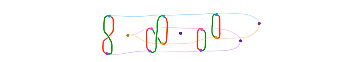
So what is \(\pi_3 \mathbf{M}O(2) := [S^3_{\mathrm{dir}},\mathbf{M}O(2)_{<4}]\)? Manifold diagrams representing functors and their transformations in \(\pi_3 \mathbf{M}O(2)\) are illustrated in Figure 8; these are simply (tamely and generically) embedded manifolds “without structure”. In particular, we give three examples of stratifications representing functors, and one example of a cobordism representing a transformation; for simplicity we omit depicting blue background squares for the stages of the cobordism (note that the transformation runs between the trivial functors, as it starts and ends in the “empty” manifold 3-diagram). The latter cobordisms, as a manifold, is an embedding of real projective space \(\lR P^2\) in \(\lR^4\) (which is a non-orientable manifold; for comparison, see the next example).
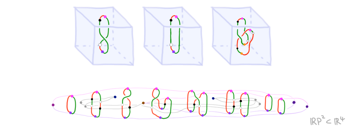
To diagrammatically compute \(\pi_3 \mathbf{M}O(2)\), note first that all occurences of \(p^\ast c^1_{0,1}\) and its inverse (i.e., the black and white dots) in a diagram can be eliminated by an appropriate cobordism (using invertibility and \(p^\ast c^2_{0,2}\)). Thus, \(\pi_3 \mathbf{M}O(2)\) must be a quotient of \(\pi_3 S^2\). In fact, via the \(4\)-cell \(p^\ast c^2_{1,1}\) it contains a cobordism that equates \(1 = 0\) in \(\lZ\): namely, by the cobordism shown in Figure 9 (again we omit depicting blue background squares for the stages of the cobordism). Thus \(\pi_3 \mathbf{M}O(2) = 0\).
This of course (via the classical PT construction) simply reflects that each 1-manifold (in \(\lR^3\)) is cobordant to the empty manifold. \(\blacklozenge\)
Example 5 (Oriented smooth manifolds). Let us next consider the Thom space associated to the special orthogonal group \(SO(2)\). By the classical PT construction, the third homotopy group \(\pi_3\mathbf{M}SO(2)\) will correspond to \(\Omega^{\mathrm{or}}_1(\lR^3)\), that is, to oriented smooth 1-manifolds \(M\) embedded in \(\lR^3\) up to oriented cobordism (technically, it is the normal bundle of \(M\) that is oriented, but since tangent and normal bundles are complements in \(\lR^3\), this is equivalently is an orientation of the tangent bundle). Following the above recipe, this can be categorically understood as follows. The space \(BSO(2)\) is \(K(\lZ,2)\), and thus has canonical cell structure (for its 2-skeleton) given by attaching a single \(2\)-cell to the point. Pulling cells back along the bundle \(\mathbf{M}SO(2) \to BSO(2)\), we deduce that \(\mathbf{M}SO(2) _{<4}\) has a single \(0\)-cell, a single \(2\)-cell, and a single \(4\)-cell; the resulting cell structure is shown in Figure 10.
Again, let us consider manifold diagrams representing elements in \(\pi_3 \mathbf{M}SO(2) := [S^3_{\mathrm{dir}},\mathbf{M}SO(2)]\), several of which are shown in Figure 8: these are now 1-manifold with orientation structure (blue strands are oriented downwards, red strands upwards). Importantly, our earlier example of an unoriented manifold, namely \(\lR P^2\) considered as a cobordism in \(\lR^4\), does no longer appear as a bordism in \(\pi_3 \mathbf{M}SO(2)\); verifying this is a fruitful exercise.
The diagrammatic computation that \(\pi_3 \mathbf{M}SO(2) = 0\) is similar to the orthogonal case, and a core role is again played by the cobordism trivializing \(1 \in \pi_3 S^2\) which we illustrate in Figure 12.
The computation reflects that each oriented 1-manifold (in \(\lR^3\)) is null-cobordant by an oriented cobordism. \(\blacklozenge\)
Example 6 (Framed manifolds). If we set \(G(2) = \ast\) (the trivial group), then \(BG(2)\) has a single \(0\)-cell and so \(\mathbf{M}G(2) = S^2\). Defining the corresponding computad \(S^2_{<4}\) as before, we therefore categorically recover the earlier case of normal framed manifolds. \(\blacklozenge\)
The pattern that emerges is the following: given a structure \(G(k) \to O(k)\), the computad \(MG(k)_ {<n}\) is the computad \(S^k_{<n}\) with additional cells attached above dimension \(n\) and as such receives a canonical map \(S^k_{<n} \into \mathbf{M}G(k)\); conversely, the map \(G(k) \to O(k)\) gives a canonical map \(\mathbf{M}G(k) \to \mathbf{M}O(k)\), and means that each \(\mathbf{M}G(k)\)-labelled manifold diagram can be turned into a \(\mathbf{M}O(k)\)-labelled one. In other words, framings are the “initial” structure, while orthogonal structure is the “terminal” structure on manifolds: this is graphically illustrated in the table in Figure 13.
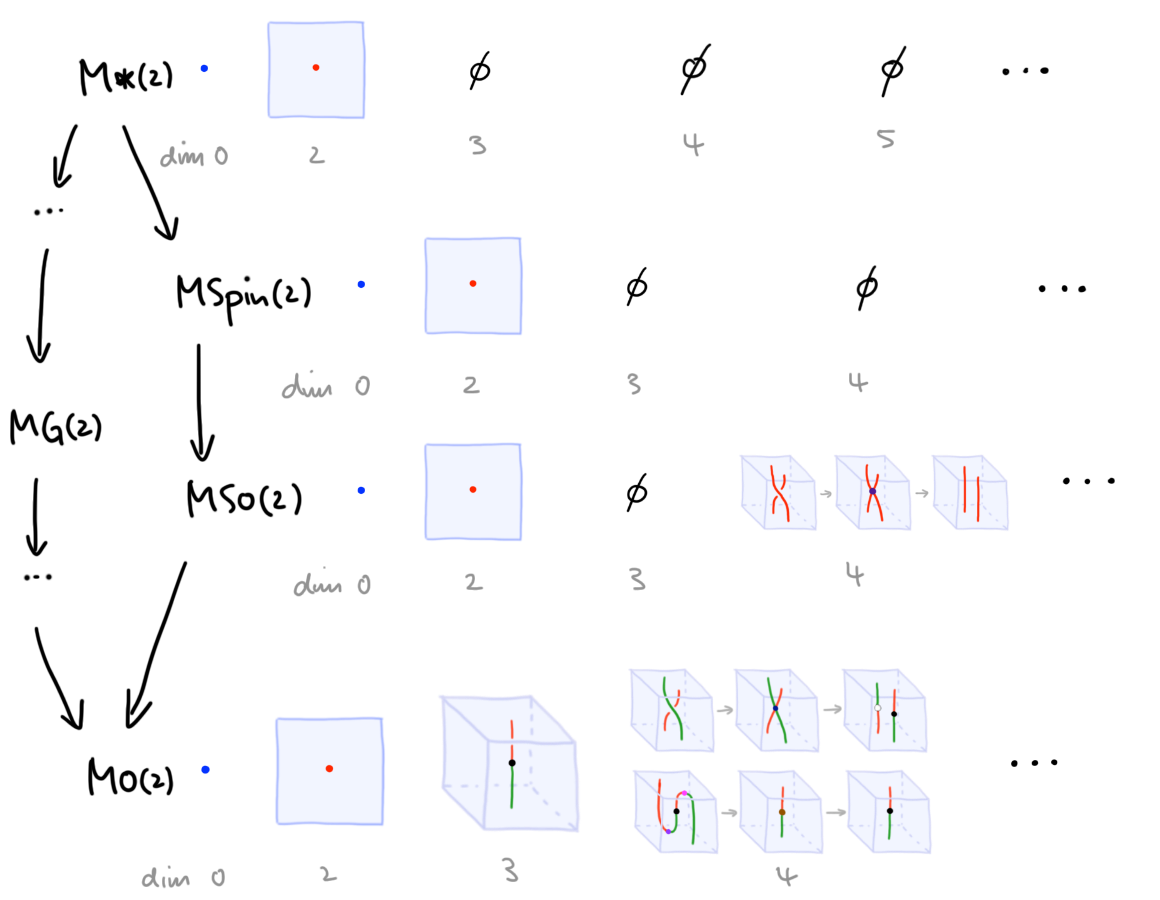
Example 7 (Non-trivial 1-manifold cobordism groups). We’ve seen \(\pi_3\mathbf{M}SO(2) = \pi_3\mathbf{M}SO(2) = 0\). From Figure 13 it is easy to see that \(\pi_3\mathbf{M}\mathrm{Spin}(2) = \pi_3 S^2 = \lZ\). This stabilizes to give the usual result:
\[\Omega^{\mathrm{Spin}}_1 = \lim_{k \to \infty}\pi_{k+1}\mathbf{M}SO(k) = \lim_{k \to \infty} \pi_{k+1} S^k = \lZ_2.\](Note \(\lZ_2 = \lZ_{/\{-1 = 1\}}\): in \(\pi_4 S^3\) the generator, now a 1-tangle in \(\lR^4\), becomes isotopic, i.e. cobordant as a manifold diagram, to its own inverse.) \(\blacklozenge\)
Generalized cohomology theories via stratified cobordism
Having come so far it would be a shame to not mention the following connection with a previous project of Buoncristiano, Rourke and Sanderson. Cobordism homology theories are homology theories that compute
\[[S^{n+k},X_+ \wedge \mathbf{M}G(n)]\](this recovers our previous discussion if we evaluate on the point \(X = \ast\)). Dually, cobordism cohomology theories are cohomology theories that compute
\[[S^{n} \wedge X_+, \mathbf{M}G(n+k)].\]As we’ve seen (via the categorical PT construction), the spaces \(\mathbf{M}G\) have the property that functors into \(\mathbf{M}G(n)\) yield stratifications of the domain’s \(m\)-cells by \((m-n)\)-manifolds with \(G(n)\)-structure on their normal bundle (up to cobordism). What does the PT construction yield for other, more general (co)homology theories? In this case it yields stratified manifolds up to stratified cobordism.
To define such “other” theories we take the abstract perspective that cohomology theories are described by hom data in \(\infty\)-toposes: in particular, any space \(T\) defines a “cohomology theory” \(\mathrm{Hom}(-,T) : \infty\mathrm{Grpd} \to \infty\mathrm{Grpd}\) (of course, in reality one’s goal is to find those theories \(T\) for which \(\mathrm{Hom}(-,T)\) is both sufficiently non-trivial and computation-friendly). Nonetheless, from this general perspective, generalized cohomology theories (evaluated on manifolds \(X\)) have the following PT interpretation.
Proposition (VII.4.1 in [5]). There is a 1-to-1 correspondence between homotopy classes of maps \([X, T]\) and cobordism classes of “framed \(T\)-manifolds” embedded in the manifold \(X\). \(\blacklozenge\)
Here, “framed \(T\)-manifolds” means what you’d expect it means (and is, to some extent, explained in the reference). BRS, using the notion of “mock bundles”, further generalize this result to the case where \(X\) need not be a manifold itself but can be an arbitrary cell complex.
This is of course analogous to what we’ve seen in the context of the categorical PT construction: given a computad \(T\) (modeling, say, some CW complex), then \([X,T]\) is exactly the \(T\)-cobordism classes of \(T\)-stratifications of \(X\). In comparison to the above result, the immediate observation is the following: in categorical terms, we need not appeal to PL (or smooth) technology of any kind to prove such generalizations of the PT construction—instead, the categorical PT construction is pretty much a tautology and moreover it applies to all computads \(X\) and \(T\) from the get-go. It is also interesting to, more specifically, compare the two approaches in the case of Thom spectra which BRS discuss in Example VII.5.3(4).
The combinatorialization of smooth structures
One upshot of our discussion here is that manifold diagrams should be able to represent smooth manifolds and their smooth cobordisms which, owing to the combinatorial nature of manifold diagrams, we refer to as the “combinatorialization of smooth structures”. Indeed, we have seen that a functor from an \((n+k)\)-cell to \(\mathbf{M}O(n)\) produces, via the categorical PT construction, a manifold diagram (up to manifold diagram isomorphism) which can be thought of as representing a single \(k\)-manifold embedded in \(\lR^{n+k}\)—by analogy with the classical PT construction, this manifold should have a unique smooth structure. There are several points that need clarification in this claim (and eventually proof). Let us unravel some of these points.
First, recall the notion of “tame embeddedings” (as previously discussed in the context of tame tangles): an embedding \(X \subset \lR^{n}\) of a manifold (or a stratified space) \(X\) is said to be tame if there exist a manifold \(n\)-diagram that refines the stratification \(X \subset \lR^{n}\). In this case, there always exists a coarsest manifold diagram refining \(X \subset \lR^{n}\) (which is coarser than all other manifold diagrams refining \(X \subset \lR^{n}\)). When we refer to \(X \subset \lR^{n}\) “as (represented by) a manifold diagram” we usually mean this coarsest manifold diagram.
Second, recall that the notion of “isomorphism of manifold \(n\)-diagrams” is defined by framed stratified homeomorphisms. Such isomorphisms can change the diagram without changing its “categorical content”; they are allowed to shift and shear strata, without changing how strata are (globally) positioned with respect to the framing of \(\lR^n\). A good analogy is with Morse functions: every manifold \(n\)-diagram comes with a projection to \(\lR^1\)—think of it as a Morse function for now, even though it might not be “generic” enough. An isomorphism of manifold diagrams will preserve this Morse function up to a (framed) reparametrization \(\lR^1 \iso \lR^1\), and it will thus preserve the order and type of 1-Morse singularities. (The isomorphism simultaneously also preserves projections of the diagram to \(\lR^k\).) Finally, we may also think about isomorphisms dually in terms of pasting diagrams of computadic cells: isomorphisms can be thought of as changing (framed) attaching maps of cells up to (framed) homotopy, but without changing the global cell structure.
In our discussion of the categorical PT construction we so far worked purely combinatorially; however, the words “up to framed stratified homeomorphism” must come into play when we realize combinatorial manifold diagrams as geometric ones; recall, combinatorial manifold diagrams correspond to geometric manifold diagrams precisely up to framed stratified homeomorphisms (see also Remark 4 above). Motivated by the correspondence of functors from a single \((n+k)\)-cell to \(\mathbf{M}O(n)\) with combinatorial manifold diagrams representing \((n+k)\)-embedded \(k\)-manifolds, we now conjecture the following.
Conjecture 1 (Manifold diagrams encode smooth structures). Given tamely \((n+k)\)-embedded smooth \(k\)-manifolds \(M^k \into \lR^{n+k}\) and \(N^k \into \lR^{n+k}\) which are framed stratified homeomorphic, i.e. they are represented by the same combinatorial manifold diagram, then \(M^k\) and \(N^k\) are diffeomorphic, i.e. carry the same smooth structure. \(\blacklozenge\)
An equivalent, catchy way of expressing this conjecture is: \(n\)-Morse functions detect smooth structures (while \(1\)-Morse functions cannot). The natural next conjecture is that all smooth structures can be encoded in this way.
Conjecture 2 (All smooth structures are encoded in manifold diagrams). Tame embeddings are dense in the set of (sufficiently compact) smooth embeddings \(M^k \into \lR^{n+k}\); in other words, any smooth embedding can be slightly perturbed to obtain a tame smooth embedding. \(\blacklozenge\)
Both Conjecture 1 and 2 have been first stated in [6].
Let’s be speculative and take this a step further: we want to get an idea about what manifold diagram singularities can appear in a diagram that represents the embedding of a smooth manifold. We will say a tame embedding \(M^k \into \lR^{n+k}\) of a manifold \(M^k\) has smooth structure if, up to framed stratified homeomorphism, it is a smooth embedding \(\tilde M^k \into \lR^{n+k}\) of a smooth manifold \(\tilde M^k\) (note by Conjecture 1 \(\tilde M^k\) is unique up to diffeomorphism). Similarly, a tame tangle) will be called smooth if its underlying tame embedding \(\tilde M^k \into \lR^{n+k}\) has smooth structure.
Conjecture 3 (Smooth structures is encoded by \(\mathbf{M}O(n)\) singularities). There is a computad \(\mathbf{M}O(n)^{\mathrm{max}}\) such that a tame embedding \(M^k \into \lR^{n+k}\) of a manifold \(M^k\) has smooth structure (and uniquely so) if and only if is represented, via the PT construction, by a functor to \(\mathbf{M}O(n)^{\mathrm{max}}\). \(\blacklozenge\)
Roughly speaking \(\mathbf{M}O(n)^{\mathrm{max}}\) is obtained by gluing in cells whenever a smooth tangle singularity between any source and target morphism exists. In a way, this is the “maximal” computad model of \(\mathbf{M}O(n)\). It is more interesting to think about the “minimal” computad model. In the following, recall the notion of elementary tangle singularities, and note that the notion of perturbation has a precise meaning in the context of manifold diagram theory.
Conjecture 4 (\(\mathbf{M}O(n)\) singularities can be chosen to be elementary). We can build a computad model \(\mathbf{M}O(n)^{\mathrm{min}}\) of \(\mathbf{M}O(n)\) whose manifold diagram singularities represent elementary smooth tangles singularities. Each tame smooth embedding \(M^k \into \lR^{n+k}\) can be perturbed to one obtained (via the PT construction) from a functor to \(\mathbf{M}O(n)^{\mathrm{min}}\). \(\blacklozenge\)
This conjecture holds for our earlier example of the \(4\)-computad \(\mathbf{M}O(2)_ {<4}\): the three cells shown in Figure 7 represent (after forgetting their stratification) elementary smooth tangle singularities. (All other singularities of \(\mathbf{M}O(2)_ {<4}\) are those that are part of adjoint equivalence data, and those singularities too are elementary smooth.)
Importantly, the class of (elementary) smooth singularities is different from the class of all (elementary) singularities. Indeed, our definition of tangle singularity only required its link to be a (PL) sphere. Thus, tamely and smoothly embedding, say, an exotic sphere \(S^k \into \lR^{n+k}\) and taking the cone of that stratification will yield a tangle singularity. Since exotic spheres (at least for \(k > 4\)) do not smoothly bound disks, and in light of Conjecture 1, this singularity cannot be smooth. However, the singularity will be “elementary PL”.
Conjecture 5 (The PL case). Appropriate variations of the above conjecture hold for the PL case.
- If tame PL embedded manifolds are framed stratified homeomorphic then they are PL homoemorphic (easy to prove actually, see [6]).
- Any PL manifold manifold has a tame PL embedding (easy to prove if manifold is compact, see [6]).
- The \((n+k)\)-computad \(\mathbf{M}PL(n)^{\mathrm{max}}\) in which cells are given by all tangle singularities of codimension \(k\) should be a model for \(\mathbf{M}PL(n)_{<n+k}\). Embedded PL manifolds can be represented by functors into \(\mathbf{M}PL(n)^{\mathrm{max}}\).
Understanding the class of elementary singularities, and the subclass of elementary smooth singularities, will provide a combinatorial description of (PL or smooth) manifold “generically” embedded in euclidean space. (Note that, in codimension \(1\), these classes coincide if the smooth 4-dimensional Poincare conjecture turns out to be true.) The combinatorial classification of elementary smooth singularities would be a first step to solve the difficulties encountered in the classical differential approach to singularity theory and higher Morse theory. We hope that future work we bring further clarity about this classification.
References
[1] “Elements of Surgery Theory”, Sadykov
[2] “Lectures Notes on Algebraic Topology”, Davis + Kirk
[3] “Characteristic Classes”, Milnor + Stasheff
[4] “Associative \(n\)-categories”, Dorn
[5] “A Geometric Approach to Homology Theory”, Buoncristiano + Rourke + Sanderson
[6] “Framed Combinatorial Topology”, Dorn + Douglas